Daily AI Digest — 2026-11-02
arXiv Highlights
ReLift: Dense 3D Tracking as Lifted Trajectory Repair
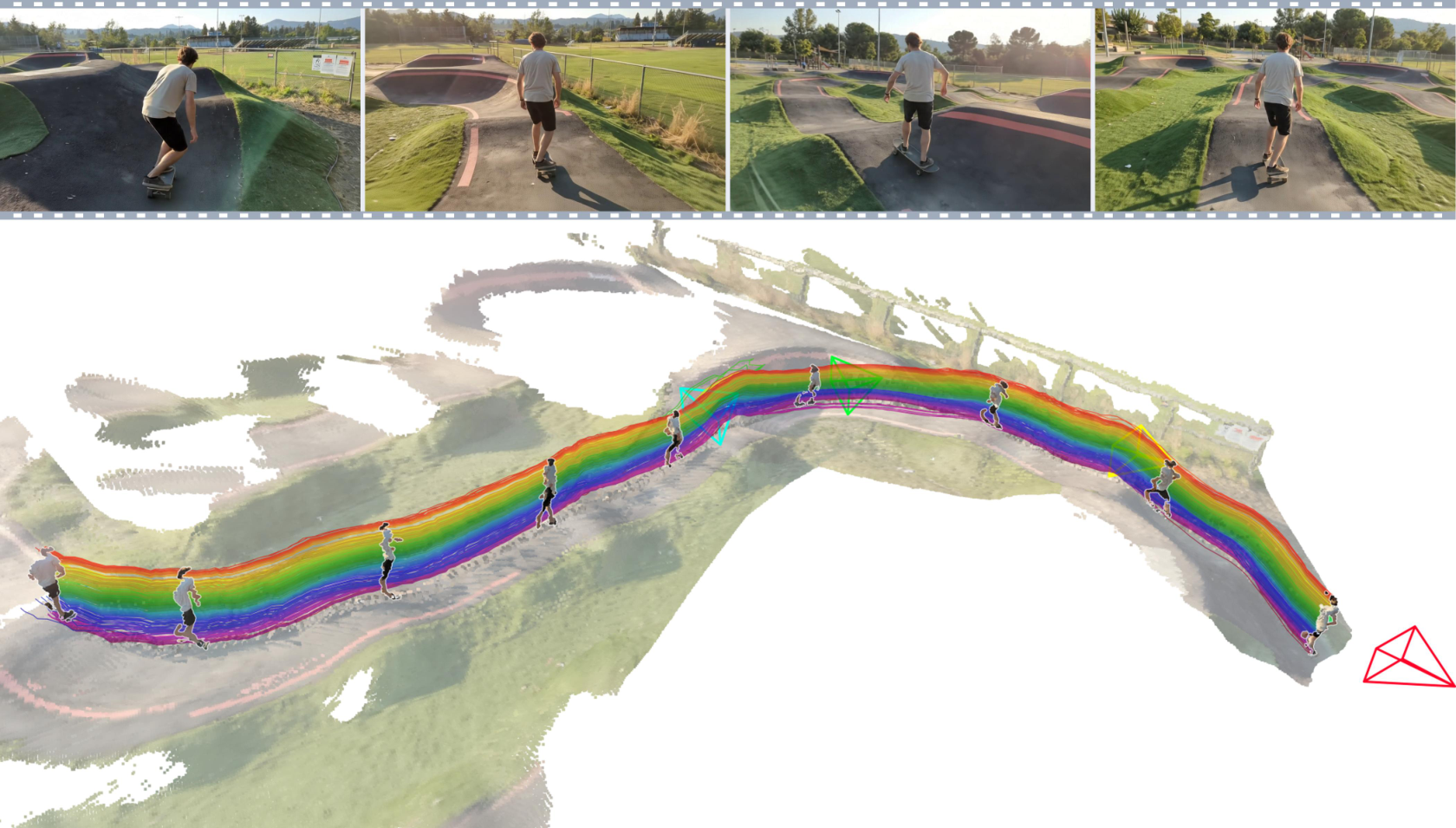
Dense 3D point tracking from monocular video jointly entails (i) correspondence across frames, (ii) metric depth per correspondence, and (iii) plausible motion through occlusions. End-to-end 4D models are bottlenecked by the scarcity of ground-truth 4D supervision. ReLift takes the opposite stance: let frozen pretrained 2D trackers and 3D geometry predictors do the perception, and train a small purely-geometric network to repair the resulting lifted trajectories. The headline empirical claim — made visible in the teaser — is that this decomposition achieves state-of-the-art accuracy on WorldTrack while sitting on a favorable speed/accuracy frontier.
Lifting and its failure modes
Given a video \{I_t\}_{t=0}^{T-1}, a 2D tracker produces image trajectories \mathbf{u}_{ti} and visibilities v_{ti}\in[0,1] for reference-frame pixels i. A geometry model yields optical-axis depth Z_t, intrinsics K_t, rotation R_t from camera t to camera 0, and camera center \mathbf{o}_t. With \mathbf{q}_{ti}=K_t^{-1}\widetilde{\mathbf{u}}_{ti}, the lifted point in reference-camera coordinates is
\mathbf{d}_{ti}=\frac{R_t\mathbf{q}_{ti}}{\|\mathbf{q}_{ti}\|},\quad r_{ti}=Z_t(\mathbf{u}_{ti})\|\mathbf{q}_{ti}\|,\quad \mathbf{y}_{ti}=\mathbf{o}_t+r_{ti}\mathbf{d}_{ti}.
The \|\mathbf{q}_{ti}\| factor converts optical-axis depth to ray distance. The authors catalogue four characteristic corruption modes in \mathbf{y}_{ti}: (1) correspondence errors perturbing \mathbf{d}_{ti} laterally; (2) depth jitter (high-frequency range noise); (3) depth drift (slow systematic range bias); (4) wrong-surface samples, where occluders or boundary bleed inject the depth of the wrong object — the most pernicious failure, because the lifted point is confidently placed on a different surface. Occlusion-induced gaps are detected via visibility v_{ti} and left as missing to be completed.
Repair as alternating attention over tracklets
ReLift forms per-sample tokens \boldsymbol{\phi}_{ti} carrying the lifted XYZ, the viewing ray direction \mathbf{d}_{ti}, and availability masks, then groups them into C-frame tracklets with embeddings \mathbf{h}_{ni}. A transformer alternates attention along a track (temporal consistency, drift, jitter) and across tracks (shared rigid or articulated motion, co-visible neighbors), producing per-frame XYZ residuals that are added to the initialized trajectory.
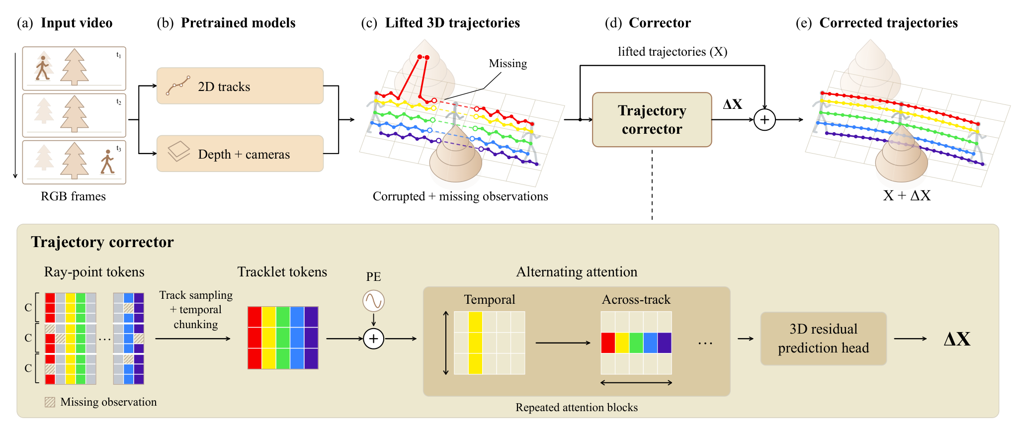
A central design decision is that the corrector consumes only geometric tokens — no image features. This has two consequences. First, inference decouples from any particular tracker/geometry backbone: swap AllTracker or VGGT-\Omega for alternatives and ReLift still applies. Second, training is cheap: the authors synthesize corrupted lifts directly from clean 3D trajectory annotations by injecting the four failure modes above, with no rendering, no 2D-tracker rollout, and no geometry provider in the loop. 4D supervision is thus concentrated on the one network that actually needs it, and the simulator can oversample rare but damaging patterns like wrong-surface jumps.
At inference, temporal chunking into C-frame tracklets and batched cross-track groups allow feed-forward correction of all reference pixels in parallel, which is what buys the FPS advantage shown in Figure 1.
Results
Evaluation is on four WorldTrack datasets — ADT and PS (real, from TAPVid-3D), and PointOdyssey and Dynamic Replica (synthetic) — scoring dense predictions at the sparse ground-truth trajectories of reference-visible points over the first 84 frames. An additional benchmark uses 50 24-frame Kubric clips from TrackCraft3R with per-reference-pixel ground truth.
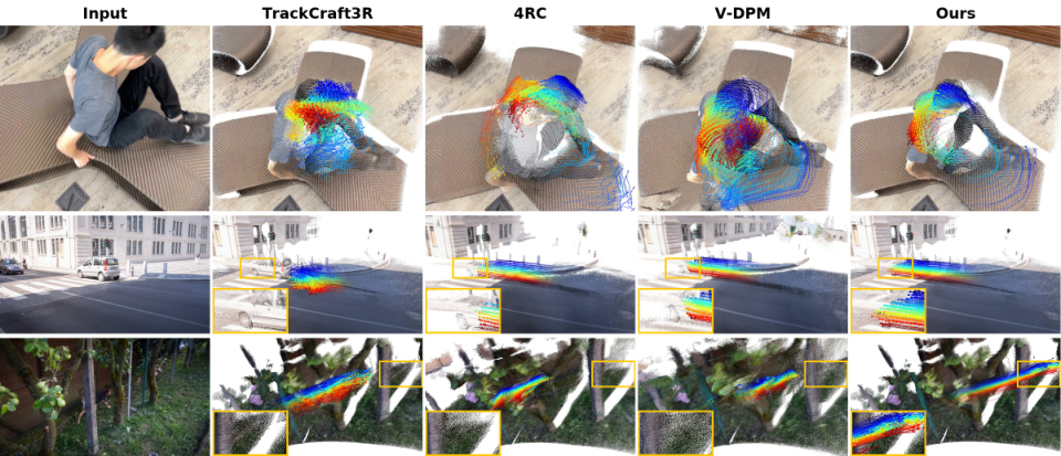
The paper’s quantitative core: a plain lift with visibility-masked interpolation already rivals purpose-built 3D trackers that share the same geometry backbone. Adding ReLift’s corrector then pushes to state-of-the-art dense 3D accuracy on WorldTrack, while keeping the full pipeline competitive on FPS (Figure 1, right). Qualitatively, trajectories from matched novel viewpoints show that ReLift fixes the characteristic failure of lifted baselines: tracks that cling to occluders rather than the occluded surface, and tracks that drift laterally at depth discontinuities.
Limitations and open questions
The approach inherits the ceiling of its providers: if the 2D tracker loses a point for the entire clip, or depth is systematically wrong at a scale the simulator did not model, there is no image signal available at correction time to recover. The simulated-lift training distribution is also a modeling choice — the fidelity of corrections depends on how well jitter, drift, correspondence noise, and wrong-surface events are parameterized to match real provider statistics. Finally, operating in reference-camera coordinates ties long trajectories to the quality of the pose estimates (R_t, \mathbf{o}_t); drift there will propagate into every corrected position. It is also unclear how much of the gain over end-to-end 4D models comes from the corrector architecture versus simply having access to much stronger 2D and geometry priors than those models were trained with.
Why this matters
ReLift makes a concrete case that 4D supervision should be spent on the thinnest possible module — a geometry-only trajectory repair network — while 2D correspondence and monocular depth remain the job of large pretrained models. This modularity lets dense 3D tracking ride future improvements in trackers and geometry estimators without retraining, and reframes “dense 3D tracking” as a trajectory-space denoising problem rather than a monolithic perception task.
Source: https://arxiv.org/abs/2610.42136
On the Origin and Evolution of Training-Inference Mismatch in LLM Reinforcement Learning
On-policy RL for LLMs is nominally on-policy only in the loss. In practice an inference engine (e.g. vLLM) samples trajectories while a separate trainer (e.g. FSDP/Megatron) computes gradients, and the two disagree. This paper decomposes that disagreement into two sources — numerical discrepancy between engine and trainer at the same weights, and policy lag from asynchronous sampling — and shows that each source demands a different correction. The authors then build DLC, a corrector that handles both.
Decomposition
At a sampled token y_t with prefix h_t, define the score s_t=\nabla_\theta \log p_\theta(y_t\mid h_t) and advantage A_t. Equation (1) splits the sampler-side update at a prefix into a drift and a covariance:
\mathbb{E}_q[a\,s] = \bar a\,\bar s + \mathrm{Cov}_q(a,s),\qquad \bar s = -\nabla_\theta \mathrm{KL}(q\,\|\,p_\theta).
The drift \bar a\bar s is a KL-step from trainer to sampler scaled by the mean prefix advantage. Because group centering only zeroes the mean advantage over a prompt — not per prefix — prefixes en route to correct answers have \bar a>0 and the drift is nonzero exactly where the learning signal lives.
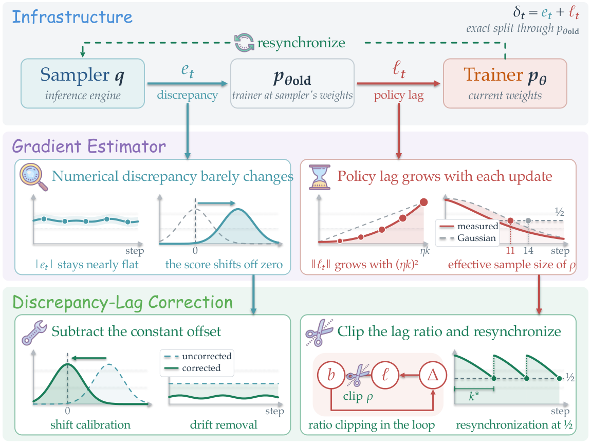
Running the trainer at the sampler’s weights \theta_{\mathrm{old}} exactly splits the per-token log-ratio \ell_t into a numerical part e_t (engine vs trainer at the same weights) and a lag part (trainer at \theta vs \theta_{\mathrm{old}}).
Source-dependence of corrections
Table 2 and Figure 2 show the asymmetry cleanly on Qwen3-0.6B over 40 steps. Deviation is measured as KL to on-policy training in units of the noise floor.
- Quantized sampler (numerical only). The discrepancy is approximately constant (~0.02 nats/token). Score centering removes the leading drift bias and recovers on-policy accuracy of 46.5%; the raw policy gradient reaches 12.7× floor and 26.4% accuracy. PPO sits at 14.3× floor.
- Stale sampler (lag only). Score centering explodes to 31.7× floor and 12.2% accuracy, while importance sampling with centering stays at 2.10× and 32.0%. PPO with the pre-batch reference reaches 699× floor.
- Combined. Importance sampling with centering handles both (2.61×, 30.5%).
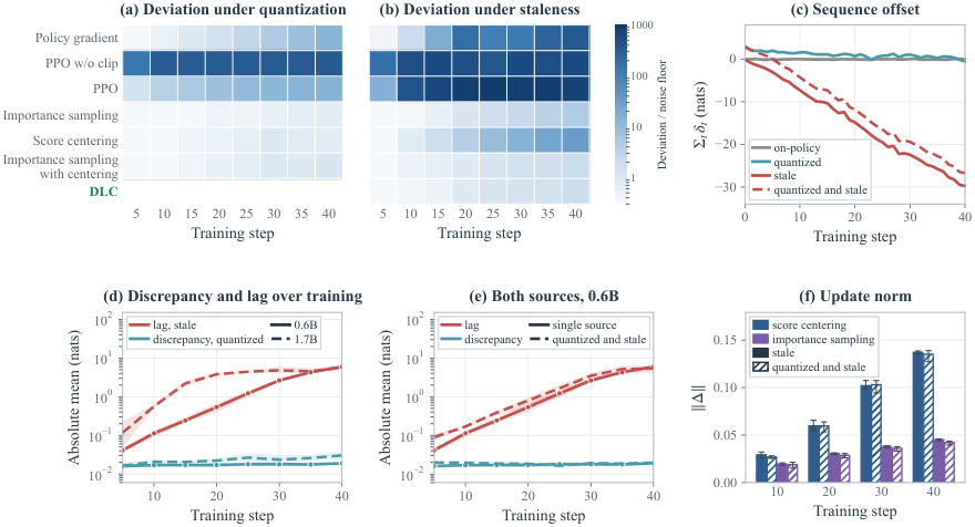
Panels (d,e) make the mechanism explicit: numerical discrepancy stays ~0.02 nats/token throughout, while policy lag grows by two orders of magnitude on both model sizes.
The lag feedback loop
Under staleness the sampler is pinned at \theta_0, so the version gap equals the accumulated update \Delta_k. The authors formalize a three-link loop — lag growth, residual bias, bias accumulation — leading to
\Delta_{k+1} \approx (I-\eta M)\,\Delta_k + \eta g_k,
where M collects the per-token weights the correction fails to remove and b_k\approx -M\Delta_k. Along eigenvectors with \lambda<0, the bias-driven component of \Delta is amplified by 1-\eta\lambda>1 each step. Empirically, the mean lag grows at 110–150× \|\Delta\|^2 for both score centering and importance sampling, so the two corrections produce the same lag per unit of movement; the difference is that importance sampling’s residual bias stays at gradient noise while score centering’s grows linearly in \|\Delta\|, driving \Delta further and closing the loop.
Where importance weighting breaks
Importance sampling cuts the loop only while the ratio \rho_t = e^{\ell_t} stays concentrated. For a Gaussian lag with mean \mu<0 (and matched variance since \mathbb{E}_q\rho_t=1), the effective sample size as a fraction of the batch is e^{2\mu}. On Qwen3-1.7B the measured ESS drops below 0.5 at step 11 with mean lag -0.15 nats/token — three steps earlier than the Gaussian prediction of -0.35 — and the deviation leaves the floor from step 11, reaching 152× by step 30. Truncation at ratio \min(p/q,2) reinstates part of the drift precisely on the tokens that most needed reweighting.
DLC
DLC assigns each failure to the layer that can fix it. Inside the algorithm:
- Run one extra trainer forward at \theta_{\mathrm{old}} to obtain \ell_t, e_t and head log-probs.
- Clip the lag ratio \rho_t=e^{\ell_t} with the standard PPO clip (\varepsilon=0.2, dual-clip c=3) against the sampler’s weights, giving weight m_t\rho_t. This is the key change from PPO: the clip reference is \theta_{\mathrm{old}}, not the pre-batch trainer.
- Subtract the sampler’s expectation of the clipped score at each prefix (score-centering generalized to the clipped estimator), splitting into reported head H and tail via \kappa=(1-\sum_H q_v)/(1-\sum_H p_{\theta_{\mathrm{old}}}(v)):
\hat g_{\mathrm{DLC}} = \sum_t A_t\,(m_t\rho_t s_t - C_t),\quad C_t = \sum_{v\in H}(q_v m_v\rho_v - \kappa p_\theta(v))\,s_v.
Lag beyond the clip’s validity range is handed back to the infrastructure via sampler resynchronization.
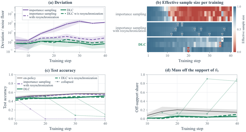
On Qwen3-0.6B under staleness, DLC reaches 1.93× floor at step 40 vs 2.10× for IS+centering and 31.7× for score centering, matching the best baseline accuracy (31.7% vs 32.0%). On Qwen3-1.7B, DLC stays at the floor where importance sampling diverges once ESS collapses, and resynchronization at the triangles in Figure 5 is sufficient to bring IS back near the floor.
Limitations
Experiments are 40-step runs on Qwen3-0.6B/1.7B; the loop analysis is first-order (b_k\approx -M\Delta_k), and the Gaussian-lag ESS prediction already deviates by three steps on 1.7B, suggesting the validity-range argument is only a leading-order guide. The resynchronization frequency is left as an infrastructure knob. PPO’s poor stale-regime behavior is attributed to using the pre-batch trainer as reference, but the paper does not test PPO with \theta_{\mathrm{old}} as reference against DLC head-to-head beyond the clip-ratio choice.
Why this matters
This paper gives the first clean operational decomposition of the training–inference gap into a (near-constant) numerical offset and a (self-amplifying) lag, explaining why GRPO, PPO, importance-sampling, and score-centering each fail in a specific regime. The DLC recipe — clip the lag ratio against \theta_{\mathrm{old}}, subtract the clipped head expectation, resynchronize when ESS collapses — is a drop-in change to verl-style stacks that any asynchronous RL-LLM pipeline can adopt.
Source: https://arxiv.org/abs/2610.40945
R^2Orch: Recursive Self-Improvement for Agent Orchestration via Self-Play within a Skill-Internalization Loop
Problem
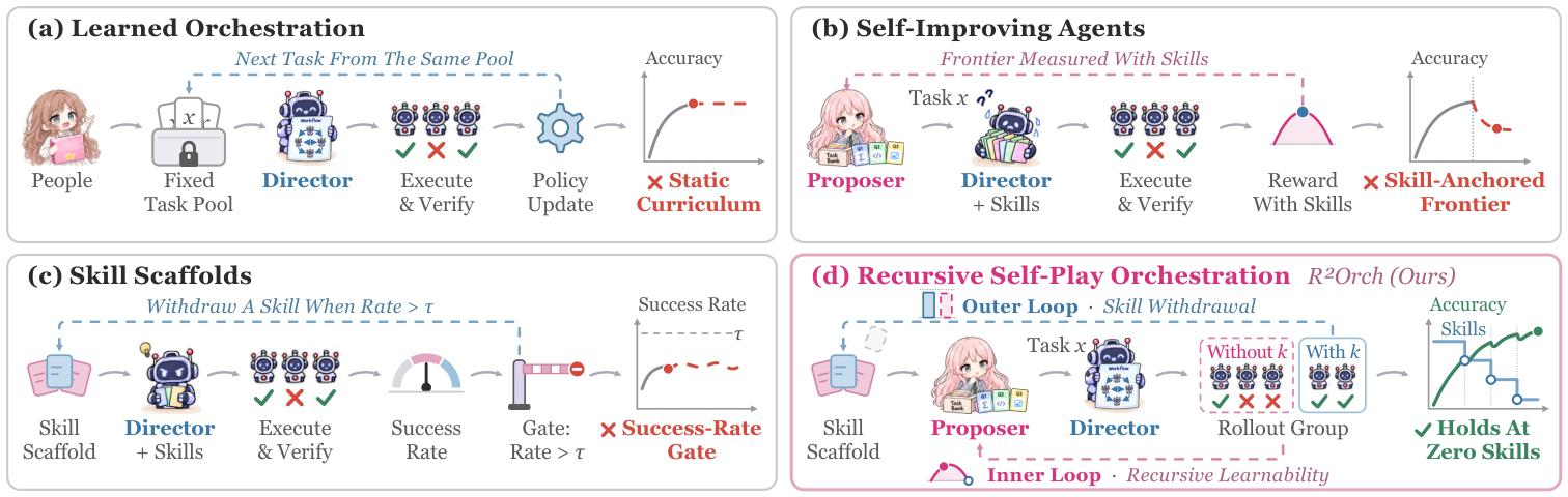
Learned orchestration of tool-using agents suffers from three coupled defects: (i) curricula are hand-designed and static, so the training distribution never adapts to what the orchestrator has already internalized; (ii) when all rollouts of a task reach the same outcome, group-relative RL methods see zero advantage and the signal collapses; and (iii) when a skill is evaluated by a single noisy success score, “does this skill still help?” is answered by a statistic the orchestrator itself contaminates via self-play. The authors frame skills (retrieved natural-language scaffolds) as training wheels that should eventually be withdrawn so that competence is pushed into parameters, not into an ever-growing scaffold.
Method
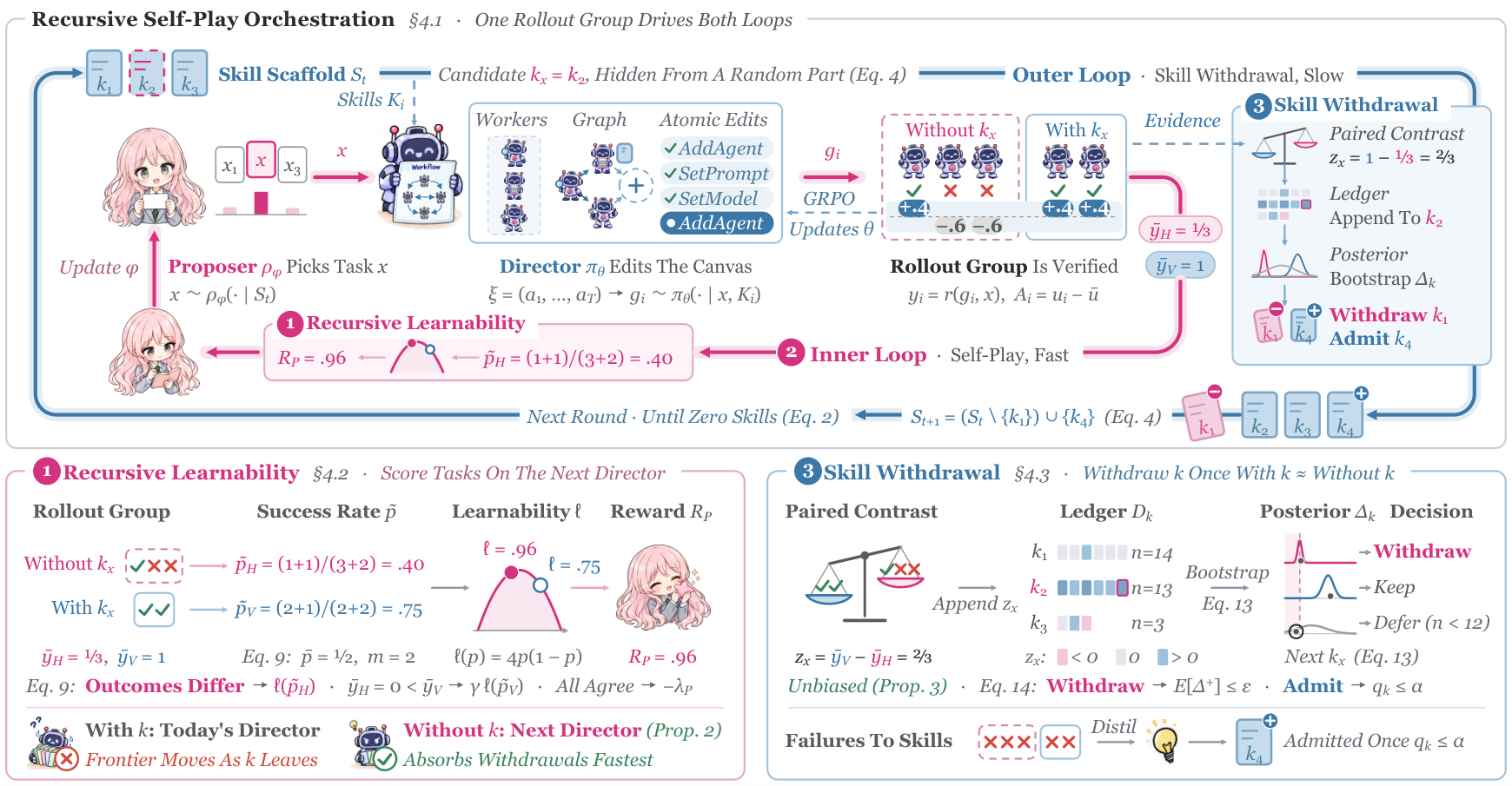
R^2Orch nests two loops joined by a single randomized rollout group of size G = n_h + n_v with n_h > n_v. In the hidden part \mathcal{H}_x a candidate skill k_x is removed from the retrieved set K_x; in the visible part \mathcal{V}_x it is kept:
q_x = \tfrac{n_h}{G}\,\delta_{K_x\setminus k_x} + \tfrac{n_v}{G}\,\delta_{K_x}.
Inner loop — Proposer/Director self-play. On the fast time scale both policies take clipped proximal best responses (two-time-scale stochastic approximation):
\theta_{t+1}\approx\arg\max_\theta \mathbb{E}\,v_K(x;\theta) - \tfrac{1}{\beta}\mathrm{KL}(\pi_\theta\|\pi_{\theta_t}),\quad \phi_{t+1}\approx\arg\max_\phi \mathbb{E}\,R_P(x) - \tau\mathrm{KL}(\rho_\phi\|\rho_0).
The Director uses GRPO with a leave-one-out baseline over the mixed-context group:
\nabla_\theta\mathbb{E}_{K\sim q_x}[v_K(x;\theta)] = \mathbb{E}\Big[\tfrac{1}{G-1}\sum_{i=1}^G (u_i-\bar u)\,\nabla_\theta\log\pi_\theta(\xi_i\mid x, K_i)\Big].
Because q_x puts most mass on K_x\setminus k_x, most of the Director update is already a no-skill update — the inner loop is pre-training itself for the withdrawal the outer loop may perform.
Recursive Learnability (Proposer reward). The Proposer is rewarded for picking x whose hidden-part rollouts (skill withdrawn) still produce mixed outcomes, i.e. tasks on the current learnability frontier after the candidate skill is removed. This directly attacks advantage collapse, since by construction 0 < \hat p_{\mathcal H} < 1 is what the reward favors.
Skill Withdrawal (outer loop). Each skill k maintains a posterior \Pi_k over the sign of its paired contrast (\mathcal V with k minus \mathcal H without k). The scaffold updates as \mathcal S_{t+1} = \Phi(\mathcal S_t;\{\Pi_k\},\mathcal F_t): a skill is withdrawn once the controlled contrast shows no benefit, and failures \mathcal F_t (groups where both parts fail) are distilled into new skills. Thus \mathcal S_t rewrites both q_x and R_P at every outer step.
Results
All ablations in Table 2 are evaluated at zero skills, so numbers reflect what has been internalized into parameters. The Qwen3.5-9B direct-prompting baseline sits at 57.81 (HotpotQA EM), 23.59 (NQ-Open), 47.19 (AIME), 15.78 (SWE), 32.81 (WebShop). GRPO-only self-play already lifts these to 86.09 / 82.97 / 73.44 / 35.00 / 71.72. The full R^2Orch reaches 91.09 / 86.09 / 90.63 / 42.81 / 91.09 — a 19.4-point gain on WebShop over GRPO-only and 27-point gain on SWE over direct prompting, with the Director holding its accuracy even though every scaffolded skill has been withdrawn (RQ3).
Component ablations isolate each mechanism. Replacing Recursive Learnability with uniform picks drops HotpotQA from 91.09 to 90.16 and WebShop from 91.09 to 87.03; with “failure reward” or DAPO-style dynamic sampling, scores land between. Replacing Skill Withdrawal with a fixed scaffold costs ~3 points on IID and 15 points on WebShop (76.09 vs 91.09), confirming the posterior-based gate outperforms success-rate thresholds (PATS), preset budgets (SKILL0), and validation gaps (SLIM).
The training-dynamics panel shows the Proposer concentrates mass on learnable (0 < p < 1) candidates and shrinks mass on already-solved ones over cycles, unlike the untrained-with-same-prompt and random baselines; the held-out accuracy at zero skills tracks accuracy with skills, i.e. skill removal does not cost competence.
Backbone transfer (RQ2) freezes the Director trained with Qwen3.5-9B Workers and swaps in six other backbones at zero skills. R^2Orch’s gains hold across code (SWE-Bench), interactive (WebShop), QA, and math-hard domains without any retraining.
Limitations and open questions
- The method depends on a reliable base retriever/skill library; distillation of failures into new skills is treated as a black box \Phi and its stability under adversarial Proposers is not characterized.
- Convergence is argued via two-time-scale stochastic approximation (Borkar, 1997), but no formal regret or non-asymptotic bound is given for the coupled Proposer/Director/scaffold triple.
- Zero-skill evaluation is the headline metric; the paper does not report cost of achieving it (rollouts, Worker calls), which matters for comparing against curriculum-free RL.
- All experiments use a single Director backbone family (Qwen3.5-9B at train time); whether Recursive Learnability’s reward remains calibrated for much weaker or stronger Directors is open.
- The paired contrast posterior assumes the visible vs hidden split is the only confound; correlated skills (one subsumes another) may stall withdrawal.
Why this matters
R^2Orch gives a concrete recipe for pushing scaffold-level competence into parameters: a mixed-context rollout group simultaneously trains the Director as if the skill were already gone and produces an unbiased paired contrast for deciding whether to actually remove it. The zero-skill numbers (e.g. 91.09 on WebShop from a 32.81 base) show that explicit “learnable-after-withdrawal” selection is a stronger curriculum signal than dynamic sampling or success-rate gating, which should influence how self-improving agent stacks are designed.
Source: https://arxiv.org/abs/2610.22740
FrameForge: Harnessing Priors of Video Foundation Models for Unified Image Generation
Problem
Unified conditional image generation — subject-driven synthesis, structure-conditioned generation (e.g., canny-to-image), and instruction-guided editing — requires a single model that preserves specific aspects of a visual input while following textual guidance. A natural idea is to repurpose pretrained video diffusion models: they already encode visual transformations across time, so conditional generation can be cast as “predict a target frame from a condition frame.” Prior work along this line typically pins the condition to frame 0 and the target to a fixed later frame, treating all tasks the same. But condition-target relationships differ sharply across tasks: an instruction edit perturbs an image slightly, a canny map is structurally close to its RGB target, and subject-driven generation can place the subject in an entirely new scene.
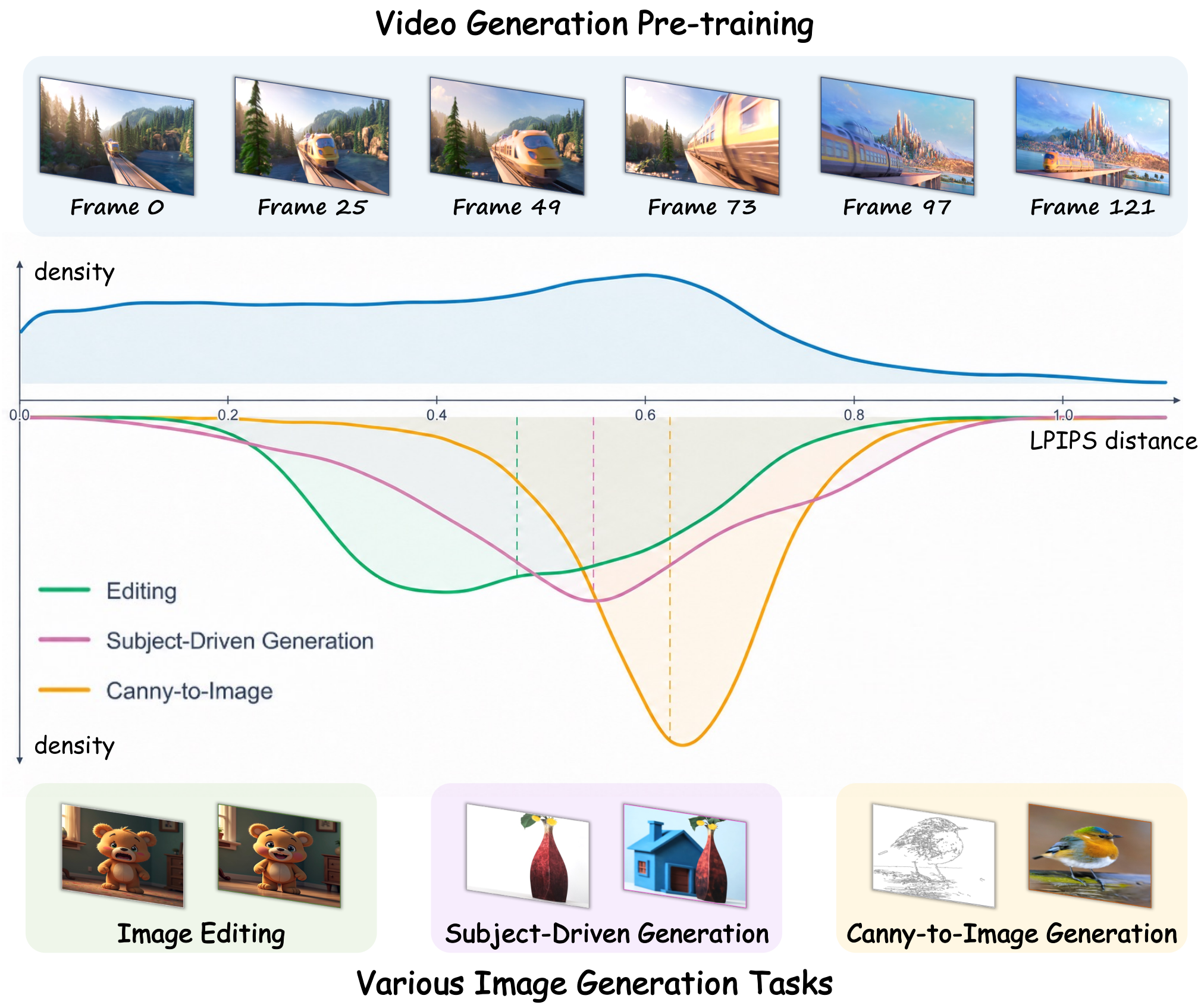
The authors quantify this by measuring LPIPS between frame pairs at varying temporal gaps in natural video and between condition-target pairs across tasks. Editing clusters near short intervals, canny-to-image at mid intervals, and subject-driven generation near large intervals — motivating an input-adaptive virtual temporal relation rather than fixed positions.
Method
FrameForge is built on HunyuanVideo1.5-T2V-720P (MM-DiT with 3D-RoPE, flow-matching loss, 3D VAE with 16\times spatial and 4\times temporal compression). The condition and target are both encoded as single latent frames; the model predicts the target’s velocity v_\theta(z_t, t, c) under
\mathcal{L}_{\text{diffusion}} = \| v - v_\theta(z_t, t, c) \|_2^2.
Two additions encode input-adaptive temporal structure.
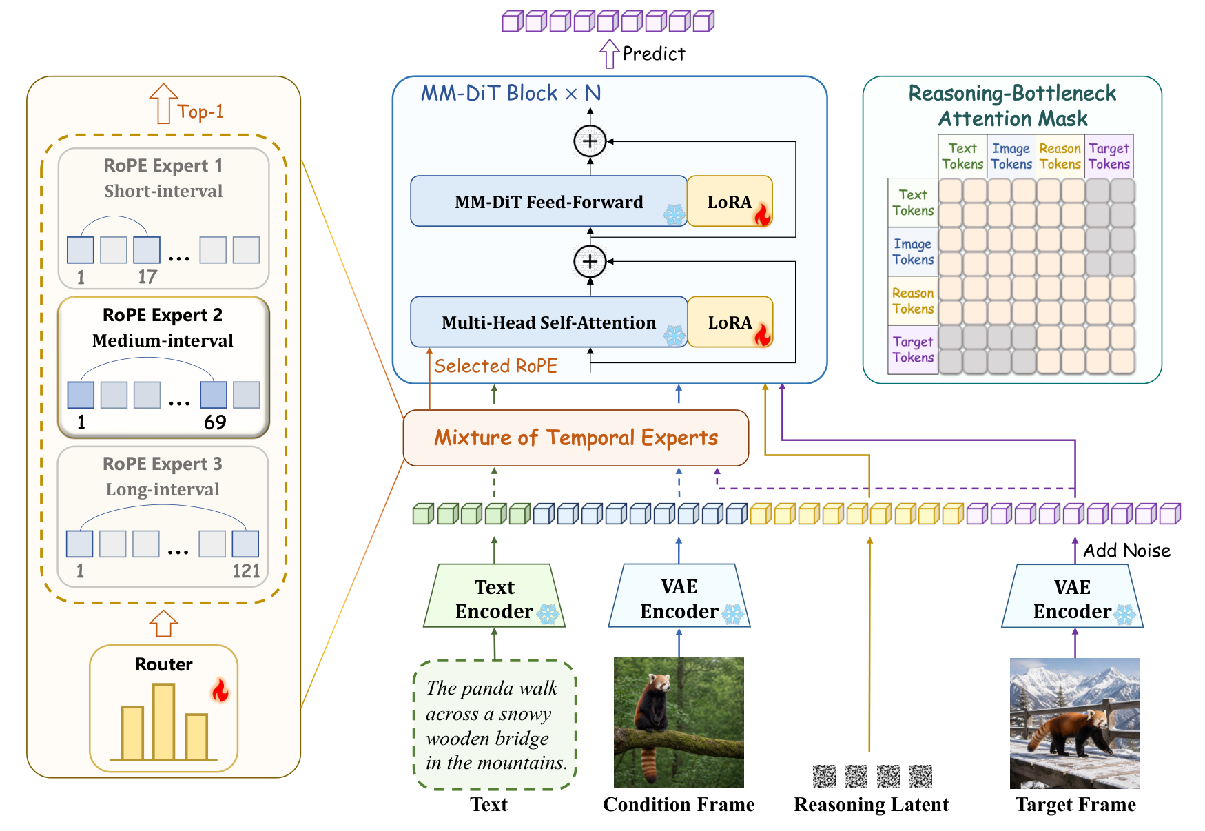
Mixture of Temporal Experts (MoTE). The temporal coordinate assigned to the target token in 3D-RoPE acts as a virtual temporal interval between condition and target. Rather than fixing this interval, MoTE maintains a bank of RoPE experts, each parameterized by a different virtual interval, and a router that chooses which expert to apply at each denoising step. The router is trained with a load-balancing loss (weight \lambda_{\text{bal}} = 0.01, softmax temperature \tau_{\text{router}} = 1.0) so that the system learns to pick small intervals for near-identity tasks like editing and larger intervals for subject recomposition.
Chain of Temporal Reasoning (CoTR). A noise-initialized intermediate latent is inserted between condition and target. Its hidden state is updated through attention and acts as a latent “midpoint frame” bridging the transformation. To force the model to actually use this pathway, intermediate-stage training applies a reasoning-bottleneck attention mask with probability p_{\text{mask}} = 0.5: this mask blocks direct text/condition→target attention, so the gradient route from guidance to target must pass through the intermediate state. Final-stage training and inference revert to full attention; the intermediate representation has by then been imprinted.
Training. LoRA fine-tuning at rank/alpha 32, giving 182M trainable parameters. Training uses 170K samples per task (510K total, filtered from Subject200K/UNO-1M, 512-2M, and HQ-Edit/UltraEdit subsets of GPT-Image-Edit-1.5M), 512\times 512 resolution, batch 60, lr 3\times10^{-4}, 12k iterations on 2× A800 (~6 days). Inference uses 50 steps with CFG scale \omega = 6 for subject/editing and \omega = 2 for canny.
Results
Evaluation covers three benchmarks:
- DreamBench (subject-driven, 30 subjects × 25 prompts, VIEScore with GPT-4o): reports SC, PQ, O.
- COCO2017 val (5,000 images, canny-to-image, GPT-4o captions): FID, SSIM, CLIP-T.
- GEdit-Bench English (606 samples, 11 categories): G-SC, G-PQ, G-O using GPT-4.1.
The excerpt provided does not include the full numerical tables, but qualitative DreamBench comparisons show the method preserves instance-level attributes (e.g., texture, structural identifiers of the reference subject) while re-rendering the subject into the prompt-specified scene.
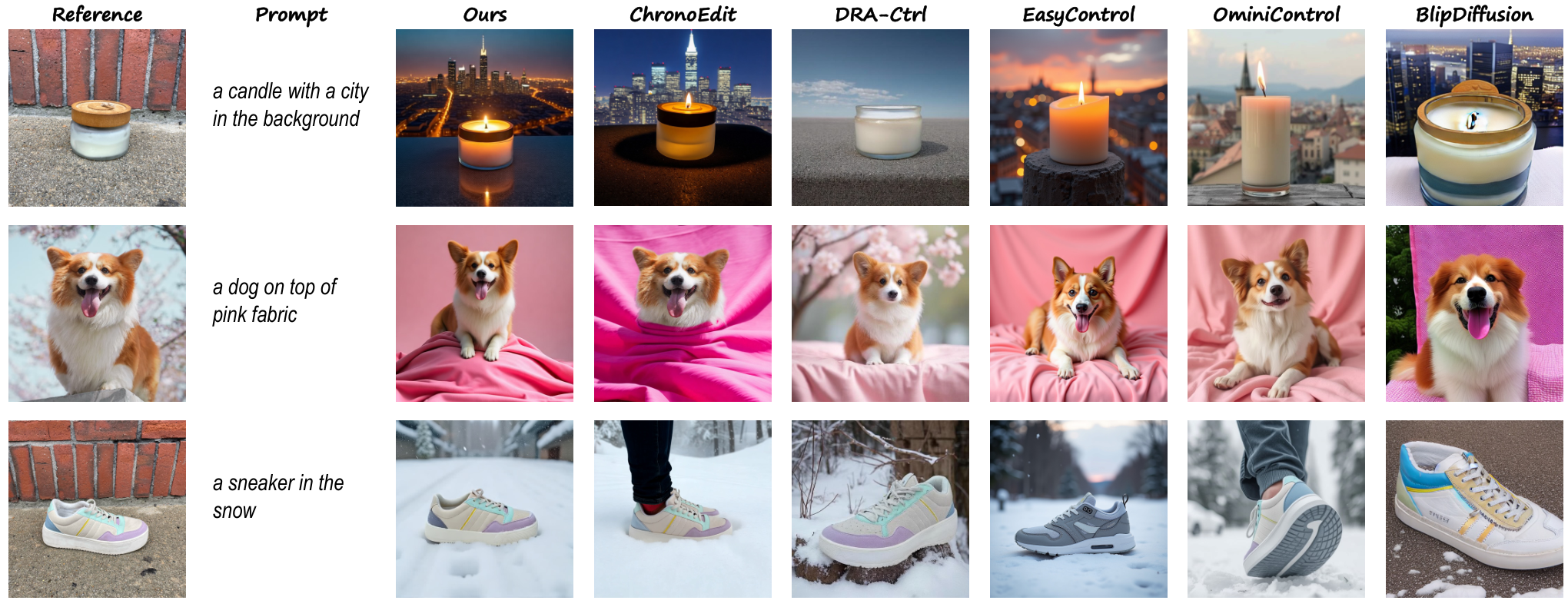
Key implementation numbers worth noting for reproduction: 182M LoRA parameters on top of HunyuanVideo1.5, 510K total training pairs equally split across three tasks, and the asymmetric CFG scales (\omega=6 vs. \omega=2) that reflect how much structural fidelity vs. semantic rewriting each task demands.
Limitations and open questions
The method is tied to a video-diffusion backbone whose compute footprint is heavier than image-only DiTs. MoTE’s expert bank size and the specific virtual intervals are design choices that likely interact with task mix; generalization to unseen condition modalities (depth, segmentation, multi-reference) is not addressed in the shown sections. CoTR’s intermediate latent is a single token-set — whether chaining multiple intermediates improves long-range transformations (e.g., multi-step edits) is an open question. Finally, routing is per-denoising-step but not spatially localized; tasks with mixed local/global changes (localized edits inside a scene swap) may want token-level routing.
Why this matters
Treating conditional image generation as adaptive-interval frame prediction gives a principled way to unify tasks whose condition-target distances differ by orders of magnitude in perceptual space, and it exploits priors already baked into video foundation models rather than training a bespoke image-conditioned architecture. The MoTE + CoTR recipe is a lightweight (LoRA-scale) retrofit, which makes it a plausible template for turning any pretrained video DiT into a general-purpose conditional image generator.
Source: https://arxiv.org/abs/2610.36545
Latent Reasoning in Continuous Space for Unified Multimodal Models
Unified Multimodal Models (UMMs) that handle both image understanding and generation typically bolt a chain-of-thought (CoT) prefix onto the generation path: the model emits discrete reasoning tokens, then conditions image synthesis on them. The authors argue this is a modality mismatch — reasoning lives in a discrete token simplex while image generation is driven by continuous latents — and that the discrete bottleneck is why reasoning-augmented UMMs (e.g., Uni-CoT) fail to inherit the test-time scaling behavior LLMs show. LARC proposes to reason directly in the continuous hidden-state space of the UMM itself, feeding the last hidden state back as the next input embedding instead of decoding to a token.
Method
LARC has two stages applied on top of a base UMM (BAGEL in the main experiments).
Stage 1 — Curriculum SFT. The model is first trained to produce textual CoT between prompt and image, then progressively more of that CoT is replaced by latent thoughts: positions where the model consumes its own last hidden state h_t as the next input embedding e_{t+1} = h_t rather than embedding a sampled token. The curriculum anneals the fraction of latent-vs-token positions, so the UMM learns to carry reasoning through continuous activations without ever being supervised on an intermediate discrete target.
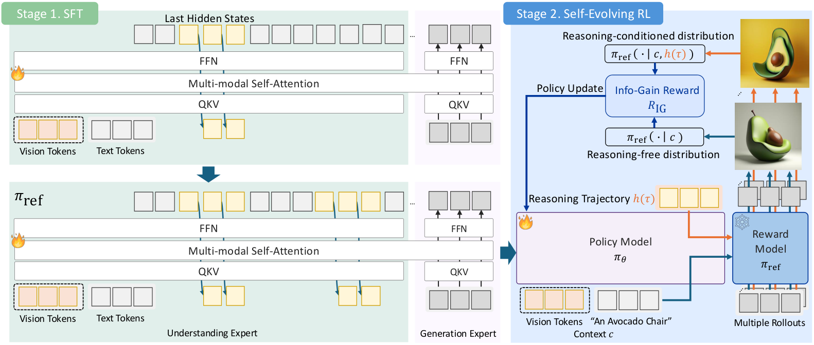
Stage 2 — Information-gain RL. Because latent thoughts have no ground-truth supervision, LARC uses a reward derived from conditional mutual information between the latent trace z_{1:L} and the generated image x given the prompt c. Intuitively, the reward is high when adding latent steps measurably reduces the model’s uncertainty over the image distribution compared to the Stage-1 reference policy \pi_{\text{ref}}:
r(z_{1:L}, x \mid c) \propto \log \pi_\theta(x \mid c, z_{1:L}) - \log \pi_{\text{ref}}(x \mid c).
This yields a self-evolving objective: trajectories whose latent reasoning carries more image-relevant information than the SFT baseline are reinforced, with no human-labeled rationales or external reward model.
Results
LARC is trained on a fixed 1M-example CoT corpus assembled from FLUX-Reason, WEAVE, and ScaleEdit, and evaluated on GenEval, DPG-Bench, OneIG-Bench (T2I), CompBench (editing), and MME/MMB/MMMU/MIRA (understanding).
On GenEval, the headline gain is Attribute Binding, where LARC improves +15 percentage points over the BAGEL base — the subtask most dependent on compositional planning, which is consistent with the hypothesis that continuous reasoning helps bind attributes to referents before pixels are committed.
On DPG-Bench, overall score moves from 85.07 to 90.04 (+5.8%), and on OneIG-Bench LARC gains +10.2 percentage points over BAGEL. The improvements are reported as consistent across every subcategory, suggesting the latent-reasoning path is not specialized to one prompt family.
On CompBench image editing, LARC posts LC-T 22.509 / LC-I 0.880 / PSNR 25.710 / SSIM 0.953 / LPIPS 0.049, dominating BAGEL (20.434 / 0.842 / 24.370 / 0.917 / 0.069), Show-o2, Emu3, Janus-Pro, and the reasoning-augmented Uni-CoT (20.215 / 0.837 / 23.925 / 0.904 / 0.088) on every metric. Notably Uni-CoT is worse than its base BAGEL on several editing metrics, reinforcing the paper’s claim that discrete CoT can actively hurt generation-side fidelity.
The more interesting result is test-time scaling. Varying the number of latent reasoning steps L at inference, LARC’s quality rises monotonically and outpaces best-of-N sampling at matched compute on T2I, editing, and visual reasoning (MIRA).
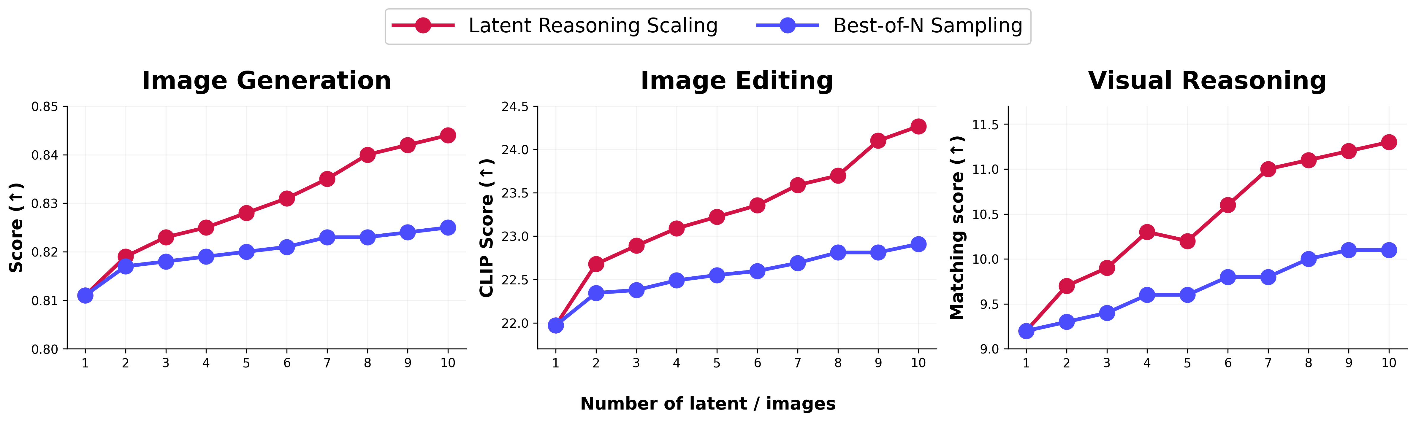
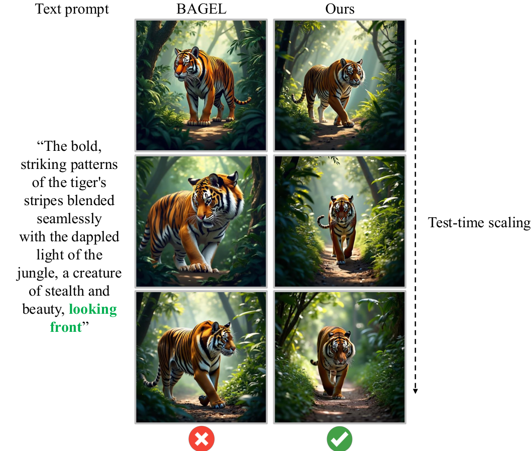
Qualitatively, at N{=}L{=}1 BAGEL and LARC are comparable, but as N,L grow to 4 and 10, BAGEL’s best-of-N outputs plateau while LARC’s latent reasoning progressively refines spatial layout and attribute binding.
Limitations and open questions
The reported experiments are built on a single base model (BAGEL); whether the curriculum SFT schedule and MI reward transfer to other UMM backbones (autoregressive-only like Janus-Pro, or MAR-style) is untested here. The information-gain reward relies on \pi_{\text{ref}} as a density baseline, so pathologies in the Stage-1 model will propagate as reward-hacking opportunities. The latent trace is also uninterpretable by construction — there is no way to inspect what the model is “thinking” at step t — which complicates debugging and safety analysis compared to textual CoT. Finally, the test-time scaling curves are shown up to L{=}10; it is unclear whether gains saturate, and the compute cost per latent step is identical to a decoder token, so the comparison to best-of-N should be read as matched-forward-passes rather than matched wall-clock given KV-cache differences.
Why this matters
LARC is a clean demonstration that the “reason in tokens, then generate pixels” pipeline is the wrong abstraction for UMMs: moving reasoning into the model’s own continuous activation space both improves generation quality and, more importantly, recovers the LLM-style property that spending more inference compute on reasoning monotonically improves outputs. If the result generalizes beyond BAGEL, latent CoT becomes the default scaling axis for multimodal generation.
Source: https://arxiv.org/abs/2610.42149
CaPtain: A Pipeline for Post-Training Code-as-Policy Robot Agents
Code-as-policy (CaP) framing turns robot manipulation into a code-generation problem: the policy emits Python against a robot API, reads back receipts, and iterates. In other agentic domains (coding, web, tool-use), the standard recipe — SFT to learn the interface, then multi-turn RL to master it — has become routine. CaP has not followed suit. Existing CaP systems either prompt frontier closed models, offload the hard part to pretrained VLAs plus high-level skills, or fail outright when a small open VLM is dropped in. CaPtain closes this gap: an open post-training pipeline that turns a small VLM into a competent CaP agent operating purely through low-level primitives, without VLAs, frontier models, or privileged state at test time.
Harness, SFT, and multi-turn RL
The pipeline has three coupled components: a fixed execution harness that defines the action and observation interface, SFT on synthetic trajectories to align the base model to that interface, and multi-turn RL that optimizes closed-loop behavior inside the same harness.
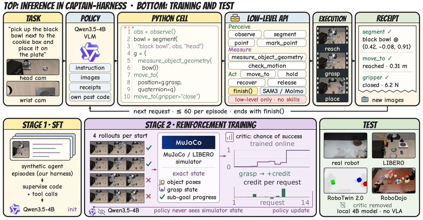
CaPtain-Harness exposes low-level perception, geometry, and guarded-motion primitives, so the same code can run in simulation and on real hardware. A task is specified by a natural-language instruction together with a TASK.md describing the API, coordinate frames, and success criterion. An episode is a ReAct loop of up to T \leq 60 requests. At request t, the policy observes
h_t = (\ell, o_1, a_1, o_2, \dots, a_{t-1}, o_t),
where \ell is the task description with initial head and wrist images, a_k is the model’s output (reasoning plus one or more Python tool calls), and o_k is the harness return (cell results, textual receipts, new images). Each request is a single model call: a_t \sim \pi_\theta(\cdot \mid h_t). The harness executes code cells in order, appends receipts and images as o_{t+1}, and reissues the next request. The loop ends when a reply contains no tool call — normally after finish() — or when a budget on requests, physical actions, or wall time is exhausted.
SFT uses synthetic trajectories generated by a stronger reference model (described as GPT-6 Astra in the abstract) rolled out inside the same harness. Because the harness is fixed, the SFT distribution and the deployment distribution share tokens, API signatures, receipt formats, and image framings — a form of in-harness alignment that avoids the usual interface drift between imitation data and the live tool-use loop.
The RL phase is multi-turn and must solve a credit assignment problem that is harder than in text agents: physical effects of a request may only manifest several turns later (e.g., a bad grasp aligned at turn t shows up as a drop at turn t+5). CaPtain uses a simulator critic that reads privileged physical state during training to produce per-request credit, and the critic is removed at test time. The policy at inference sees only receipts and images.
Experimental setup
Training is limited to the 40 original LIBERO tasks. Evaluation spans LIBERO (official held-out initial states 11–16 for all 40 tasks, 240 episodes) and three perturbation suites that never appear in training: LIBERO-PRO (object-position and task-semantics perturbations across Spatial/Object/Goal/Long; 100 episodes per subset, with reported 3-suite average over 600 episodes and 4-suite average over 800 episodes), LIBERO-Plus (stratified 700 cases over seven perturbation dimensions), and LIBERO-MAX (80 Lite cases under Base and Dynamic in-episode perturbations). Zero-shot transfer is probed on RoboTwin 2.0, RoboDojo, SimplerEnv, and CaP-Bench.
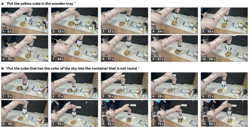
The real-robot setup adapts the policy via a twin simulation of the XR1 arm, keeping the harness identical across sim and hardware so the trained policy transfers without extra fine-tuning on real data.
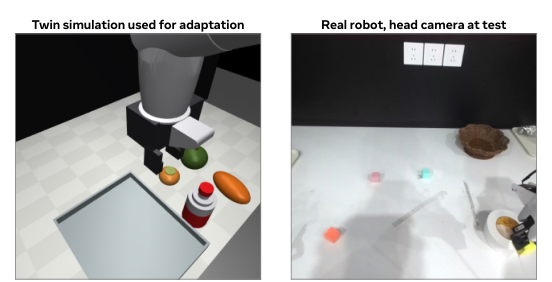
Real-robot episodes include compositions with new objects and layouts, and tasks that require language grounding: for instance, inferring that “the cube with the color of the sky” is the light-blue one and that “the container that is not round” is the rectangular tray.
Limitations and open questions
The pipeline leans on three strong priors: a well-engineered harness with reliable low-level primitives (perception, geometry, guarded motion), a stronger teacher for SFT trajectory synthesis, and access to a simulator that can be instrumented for a privileged critic. Each of these may be hard to replicate in domains where primitives are brittle, teachers are unavailable in-distribution, or privileged state is not well-defined. The 60-request budget caps episode length and effectively bounds the horizon the RL stage must credit; it is unclear how the critic scales to longer-horizon manipulation where latent effects compound further. Finally, training only on the 40 LIBERO tasks is a narrow coverage base — generalization results on LIBERO-PRO, -Plus, -MAX, and the zero-shot sims will determine how much the harness-plus-RL recipe actually buys beyond interface alignment.
Why this matters
CaPtain is the first open demonstration that the SFT-then-multi-turn-RL recipe used for coding and web agents transfers to robot manipulation when the action space is code against a low-level API, without leaning on VLAs or frontier models. If it holds up quantitatively, it reframes small open VLMs as viable substrates for robot policies, with the simulator critic as a general tool for turning privileged state into dense per-turn credit.
Source: https://arxiv.org/abs/2610.40799
REA: A Routed Embodied Agent Runtime for Asynchronous Brain-Cerebellum Control
Problem
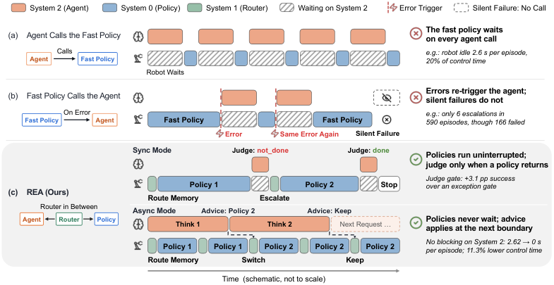
Dual-process embodied architectures — a deliberative foundation model (System 2) paired with fast reactive policies (VLAs, whole-body controllers, scripted code) — are an obvious design point, but naive couplings degrade in two symmetric ways. If the agent drives the loop and calls the policy, every control step inherits agent latency; if the policy calls the agent on errors, persistent exceptions trigger repeated fallbacks while silent failures (policy terminates “successfully” but task is unsolved) are missed entirely. The paper’s organizing constraint is a single rule: no running policy waits on the brain. The question is how to retain brain-level generalization while keeping the fast loop at native rate and still catching silent failures.
Method
REA is a runtime with three cooperating tiers: System 2 (foundation-model agent/judge), System 1 (an embodied router), and System 0 (fast policies — VLAs, code policies, WBCs). Coordination is organized around three mechanisms:
Route memory. For each task/condition, each candidate policy’s success rate is measured offline and stored. At dispatch time, the router selects a policy by looking up the measured posterior rather than querying the brain. This replaces per-episode planning with amortized evidence.
Boundary-triggered judge gate. The System 2 judge is invoked only at policy boundaries — on exception, truncation, or policy return — never mid-rollout. On a
not_doneverdict the router escalates along a ladder of alternative policies; ondonethe episode terminates. This is what detects silent failures, since a visual judge inspecting the end state does not depend on the policy raising an error.Escalation ladder. Policies are ordered (e.g., Evo → Fix → Evo again), and recovery after a judge rejection or exception advances along this ladder up to a bounded number of attempts.
Three variants instantiate the runtime: REA-M (route memory + exception gate, no online System 2), REA-A (System 2 picks initial and recovery policies), and REA-V (route memory + visual judge at returns). The variants let the authors isolate the contribution of memory, agent routing, and visual judging.
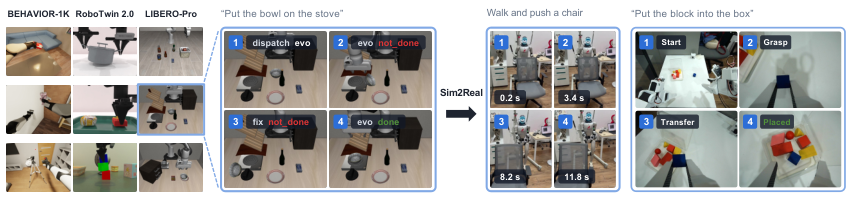
The middle panel of the above figure illustrates the silent-failure case the design targets: a bowl-on-stove episode where all three attempts terminate without exceptions, and only the visual judge distinguishes the first two failed placements from the final successful one.
Experiments
Primary evaluation is on LIBERO-Pro, which perturbs LIBERO along object/position (swap)/language/task/environment axes. The authors use the goal, object, and spatial suites under task and swap perturbations — six suites, ten tasks each, 50 seeds per task, yielding 3,000 episodes per method on the full set and 600 episodes for the cross-method study (seeds 1–10). Horizon is 4,000 steps with a 900 s wall-clock budget; routed methods are capped at three policy runs per episode. A matched hard subset of six tasks × 12 seeds (8 of which are seeds where the reference Fix policy fails) stress-tests recovery.
Portability is checked on BEHAVIOR-1K (R1Pro in Isaac Sim, five pick-up tasks), RoboTwin 2.0 (bimanual, SAPIEN, with a 100-scene VLA+code study and a 200-scene transfer study), and real Unitree G1 and AlohaMini2 platforms.
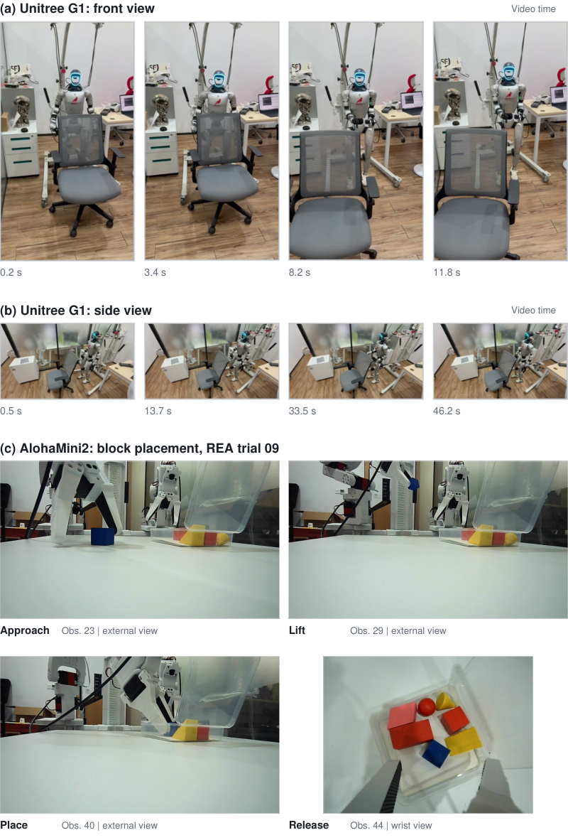
The construction of the hard subset is the key design choice for stressing the silent-failure claim: because 8/12 seeds are known Fix failures, any method that cannot escalate after a silent termination will show its true floor. The abstract and setup emphasize that the exception-triggered coupling misses silent failures entirely, which is the regime where REA-V’s visual judge should matter most.
Limitations and open questions
The excerpt provided does not pin down headline aggregate numbers across suites, so the magnitude of the improvement over the (a) agent-in-loop and (b) policy-calls-agent baselines must be read from the full tables. Several structural questions are visible from the setup: (i) route memory presumes offline success-rate estimates that are stable under the test perturbations, which may degrade as the OOD gap grows; (ii) the three-run cap and 900 s budget bound recovery depth and could favor REA on tasks where two–three policies suffice; (iii) the visual judge is itself a foundation-model call whose false-negative rate directly bounds REA-V’s ceiling, and its calibration under distribution shift is not probed in the shown sections; (iv) escalation ladders are hand-constructed from the available policy pool, so scaling to large libraries will require learned ordering.
Why this matters
REA formalizes brain–cerebellum coupling as a routing-and-gating problem rather than a planning problem, and enforces the practical invariant — the fast loop never blocks on System 2 — that makes dual-process agents usable at real control rates. The route-memory-plus-boundary-judge pattern is a transferable recipe for integrating heterogeneous policy stacks (VLA + code + WBC) without redesigning each.
Source: https://arxiv.org/abs/2610.42053
Hacker News Signals
Proving and improving the Platonic Representation Hypothesis with JEPAs
The Platonic Representation Hypothesis (PRH) conjectures that large models trained on different modalities and objectives converge toward a shared statistical model of reality — a universal representation of the world. This paper provides formal grounding for that claim and shows how Joint-Embedding Predictive Architectures (JEPAs) can be used both to test and to strengthen it.
The authors formalize the PRH in terms of mutual information and representational alignment: two encoders f_\theta and g_\phi over modalities X and Y converge if their representations maximize I(f_\theta(x); g_\phi(y)) subject to minimal sufficient statistics. They prove that under mild assumptions about data-generating processes sharing a common latent Z, any sufficiently expressive encoder trained to predict across views must recover Z up to invertible transform.
JEPAs are central because they learn by predicting latent representations rather than pixels or tokens, making them natural candidates for probing representational universality without reconstruction bias. The paper trains JEPAs on vision, audio, and text, then measures cross-modal alignment using centered kernel alignment (CKA) and nearest-neighbor consistency. JEPA representations achieve higher cross-modal CKA scores than contrastive or generative baselines, suggesting the predictive-in-latent-space objective is specifically favorable for convergence.
Quantitatively, they report CKA alignment improvements of 8-14 percentage points over CLIP-style contrastive models when comparing vision JEPAs to language model representations, and the gap widens with scale. The paper also includes ablations showing that the context masking strategy in I-JEPA is a critical variable: aggressive masking correlates with stronger convergence.
Limitations include reliance on CKA as a proxy for true representational identity, and the theoretical results require assumptions about shared latents that may not hold for genuinely disjoint domains. Whether convergence implies a useful universal representation rather than a degenerate one remains open.
Source: https://arxiv.org/abs/2610.39302
The AI cost of JavaScript frameworks
This post quantifies a previously underappreciated externality of heavy JavaScript frameworks: they inflate the token cost of AI-assisted development because LLMs must process, generate, and reason about far more boilerplate than equivalent vanilla implementations.
The author measures this concretely by taking representative UI components implemented in React, Svelte, Vue, and plain HTML/JS, then counting tokens via the OpenAI tokenizer. A simple interactive counter in React (with hooks, imports, JSX) runs around 180 tokens; the equivalent in 40 lines of vanilla JS is under 60. The ratio compounds for real applications: a small CRUD form clocks in at roughly 3x more tokens in framework code than in imperative DOM manipulation.
The implications are economic and qualitative. At current API pricing, a development session involving many round-trips over framework-heavy code costs meaningfully more. More important is the qualitative degradation: more tokens means larger context consumption, higher probability of the model losing track of earlier constraints, and more surface area for hallucinated API usage of framework-specific idioms that may be version-incorrect.
The post also notes a feedback-loop problem. LLMs trained on the web have seen enormous volumes of React code, which makes them fluent at generating it, which incentivizes developers to keep using it in AI-assisted workflows, which keeps training data skewed toward frameworks. Vanilla DOM code is underrepresented in training data, so model quality on it is paradoxically worse despite it being structurally simpler.
The author does not argue for abandoning frameworks categorically. The practical takeaway is that the token overhead should be a first-class consideration when choosing abstractions for greenfield projects expected to rely heavily on LLM tooling, and that thin wrapper libraries may offer a better cost/capability tradeoff than full reactive frameworks in that context.
Source: https://nolanlawson.com/2026/10/28/the-ai-cost-of-javascript-frameworks/
Show HN: OmniDiff – Opensource, super fast, content aware Git difftool, in Rust
OmniDiff is a Git difftool written in Rust that performs content-type-aware diffing rather than treating all files as line-delimited text. The core premise is that git diff and most frontends produce structurally meaningless diffs for non-text or structured-text formats because they operate at the byte/line level without parsing.
The implementation routes each file through a content detector that identifies format (JSON, TOML, YAML, CSV, binary, image, etc.) and dispatches to a format-specific differ. For structured data formats, OmniDiff deserializes both sides into an in-memory tree, computes a tree edit distance diff, and renders the result in a normalized, semantically meaningful form. A JSON diff, for example, shows key-value insertions and deletions without noise from whitespace reformatting or key reordering. Binary diffs show hex-level changes with context. Image diffs produce a pixel-wise delta summary.
Performance is achieved through Rust’s ownership model enabling zero-copy parsing where possible, parallel dispatch of per-file diffing using Rayon, and lazy format detection (magic bytes first, then extension, then full parse attempt). The README reports diffing a 50k-file repository with mixed content in under 2 seconds on a modern laptop, versus ~12 seconds for a Python-based equivalent.
The Git integration is straightforward: set GIT_EXTERNAL_DIFF=omnidiff or configure it in .gitconfig under [diff] external. It also supports use as a standalone CLI tool outside Git.
Current limitations noted in the repository: PDF and Office format support is planned but not yet implemented; the tree-edit-distance algorithm for very large JSON files (>10 MB) can be slow due to the quadratic worst-case of the Myers-variant used. Contributions for additional format handlers are structured around a trait interface, making extension mechanical.
Source: https://github.com/ivankovic/omnidiff
GPT-5.6 Sol can beat Factorio on peaceful mode
Factorio is a meaningful benchmark for AI planning because it demands multi-horizon goal decomposition, resource graph management, and iterative automation under scaling constraints. Peaceful mode removes combat, isolating the logistical and optimization challenge: build a factory that launches a rocket.
The author tested GPT-5.6 Sol via a Python harness that translates game state into a structured text representation and feeds it to the model as a context, then parses model output into game actions. The model is not fine-tuned on Factorio; it operates purely from in-context game state descriptions and its pretraining knowledge of the game.
The run succeeded in roughly 18 in-game hours (compressed to a multi-hour real session). Key observations: the model handles early-game resource bootstrapping competently — it knows to prioritize iron and copper smelting ratios and sets up basic automation without prompting. The mid-game transition to blue science is where prior model versions broke down due to the combinatorial complexity of balancer and splitter configurations; GPT-5.6 Sol navigates this by decomposing it into sub-goals with intermediate verification steps, asking the harness to report throughput metrics at each stage.
Failures and near-failures were documented: the model repeatedly misjudged inserter throughput limits, requiring the harness to inject a corrective error message before it replanned. It also attempted suboptimal spaghetti layouts that required backtracking. The author notes the model never once used circuit networks, which is a significant simplification since peaceful mode makes that feasible.
The result is notable not because peaceful Factorio is a hard human challenge, but because it demonstrates sustained coherent planning over hundreds of sequential decisions without retraining. The open question is whether the same approach survives deathworld settings where reactive replanning under resource pressure is required.
Source: https://ryanmadden.net/gpt-56-beats-factorio/
Postgres 19 is late because so many more bugs are being found now
Robert Haas, a PostgreSQL major contributor, writes that the Postgres 19 release cycle has slipped because the volume of bug reports has increased substantially and he attributes this directly to AI coding tools.
The technical substance of the post is about bug character, not just count. Haas observes that bugs being filed now are increasingly in obscure code paths — rare combinations of features, edge cases in type coercion, unusual planner hint interactions — that suggest code written by developers who did not deeply understand what they were writing. AI-generated SQL and PL/pgSQL tends to use valid-but-unusual syntax combinations that expose untested paths in the parser and executor. The bugs are real, but they are the kind that rarely surface when the code author understands the semantics.
This creates a compounding problem for the release process. Postgres follows a feature freeze followed by a bug-fix period before release. If the inflow rate of valid bug reports during the stabilization window exceeds the historical baseline, the window must extend. Haas notes that the committer pool has not scaled with the bug report volume, so triage time per bug has increased.
He is explicit that this is not a complaint about AI use per se — valid bugs getting found is good — but the timing asymmetry is a practical problem: the bugs are artifacts of generated code being deployed in production before the generator’s users understood the code’s implications, and they hit the database layer rather than the application layer.
The broader engineering implication is that test coverage for databases needs to anticipate AI-generated query patterns, which explore a different region of the input space than human-written queries. Fuzz testing with LLM-sampled SQL is the obvious extension.
Source: http://rhaas.blogspot.com/2026/10/postgres-19-is-late-and-its-ais-fault.html
Malware uses LLMs to rank victims by how much they’re worth
Cisco Talos has documented a novel capability in the Volta infostealer: after exfiltrating data from a victim machine, it calls an LLM API to score the victim’s financial and organizational value before deciding how much operational effort to invest in further exploitation.
The technical pipeline works as follows. Volta exfiltrates a standard package: browser-stored credentials, session cookies, crypto wallet files, clipboard history, and installed application lists. Rather than returning all this raw data to a C2 for manual review, it serializes a structured summary and sends it to an LLM endpoint (the Talos report identifies this as a commercial API, not a self-hosted model). The prompt asks the model to estimate victim value across several dimensions: likelihood of corporate network access (inferred from VPN clients, domain-joined status indicators, enterprise software), cryptocurrency holdings evidence, and presence of privileged credentials.
The model returns a priority score with a brief rationale. High-scoring victims trigger additional payload stages — persistence mechanisms, lateral movement modules — while low-scoring ones are left with only the initial credential theft to minimize operational footprint and reduce detection surface.
This is operationally significant because manual triage of infostealer logs is a known bottleneck for threat actors; automating it with an LLM removes the human-hours constraint. The model does not need to be especially accurate; even a noisy filter that correctly ranks the top decile of victims reliably is a substantial efficiency gain for the attacker.
From a detection standpoint, the LLM API call is a new indicator of compromise type: outbound HTTPS to a commercial LLM endpoint from a process that should not be making such calls. Talos recommends monitoring for this traffic pattern. The broader implication is that LLM APIs are now part of the malware supply chain.
Zombie stats: Where the numbers AI quotes come from
This post by Trakkr Research investigates the provenance of specific statistics that LLMs confidently cite — numbers like “65% of consumers prefer X” or “the average employee spends 2.5 hours per day on email” — by attempting to trace them back to primary sources.
The methodology is manual and systematic: pick a widely-cited statistic that appears in LLM outputs, search for the original study, and classify the result. The taxonomy the authors develop is: (1) sourced — traceable to a peer-reviewed study or credible primary research; (2) degraded — traceable to a real source but the number has mutated through citation chains; (3) zombie — the stated source either does not contain the number, does not exist, or the study itself was a press release or vendor survey never subjected to scrutiny.
Their sample of 200 statistics returned by GPT-4 and Claude across business, psychology, and productivity domains found roughly 38% fully sourced, 29% degraded, and 33% zombie. The zombie category includes cases where the model hallucinated an entirely plausible-sounding journal citation, but also cases where a real journal is cited but the number comes from a vendor white paper that merely referenced that journal on an unrelated point.
The degraded category is particularly interesting technically: it implies that training data contains citation chains where numbers drift — rounding, scope changes, population changes — and the model learns to reproduce the drifted number along with the original source attribution, creating a mismatch that is hard to detect without checking the source manually.
The practical implication for anyone using LLMs to generate research-adjacent content is that numerical claims require independent verification at the primary source level, not just confirmation that a plausible source exists.
Source: https://trakkr.ai/trakkr-research/zombie-stats
Show HN: I Turned DOOM into a Transformer
DoomFormer is a project that trains a transformer to autoregressively model DOOM gameplay as a sequence of discrete tokens, then uses it as a generative model for playable game states. The framing is similar to GameNGen but uses a pure transformer rather than a diffusion backbone.
The implementation tokenizes each game frame using a VQ-VAE trained on DOOM screenshots, producing a fixed codebook of 8192 visual tokens per frame at a compressed spatial resolution (roughly 20x15 patches). Game state metadata — player health, ammo, current map identifier — is prepended as special tokens. The full sequence fed to the transformer is [s_1, a_1, s_2, a_2, \ldots] where s_t is the frame token sequence and a_t is the action token.
The transformer is a standard decoder-only architecture (24 layers, 16 heads, 1024 embedding dimension) trained with a cross-entropy loss over the next-token prediction objective. At inference, the model generates the next frame’s token sequence conditioned on prior frames and the next action, then the VQ-VAE decoder renders it to pixels. The model was trained on roughly 50 hours of recorded DOOM E1M1 gameplay.
Qualitative results show the model maintains spatial coherence for several seconds of simulated play, handles door-opening events and enemy spawns with approximate correctness, and generalizes enemy positions plausibly within the trained map. Temporal coherence degrades beyond about 15 seconds of generation; the model forgets room layouts and starts hallucinating geometry.
The repository is a clean research prototype: training scripts, the VQ-VAE training code, and an inference loop that accepts keyboard input and renders frames in real time at roughly 8 FPS on a single A100. The key open problem noted by the author is the context length scaling required to model longer play sessions without the spatial forgetting.
Noteworthy New Repositories
tangency-labs/solidcraft
SolidCraft is a parametric 3D CAD application written entirely in Rust, targeting desktop, web (via WASM), and headless automation use cases. The parametric core means geometry is defined by a constraint graph — change a dimension and dependent features recompute, which is the fundamental requirement for engineering CAD as opposed to mesh sculpting tools.
The pure-Rust implementation avoids the traditional dependency on OpenCASCADE (the C++ kernel underlying FreeCAD, OpenSCAD derivatives, and most open-source CAD) — a deliberate choice that trades ecosystem maturity for memory safety, compile-to-WASM feasibility, and unified toolchain. The web target is architecturally significant: full parametric CAD in a browser without a server-side compute step has been a persistent gap.
The MCP (Model Context Protocol) integration exposes CAD operations as structured tool calls, enabling LLM-driven design automation — generating or modifying geometry programmatically through the same interface an agent would use for any MCP-compatible tool server.
At 13k stars shortly after public release, interest is high, but the project is early-stage. The core constraint solver, which is the hardest part of any parametric CAD kernel, will determine long-term viability. Anyone evaluating it should stress-test over-constrained and under-constrained sketch resolution before relying on it for production workflows.
Source: https://github.com/tangency-labs/solidcraft
opengeos/RustGIS
RustGIS is a full GIS desktop application written in pure Rust, covering the standard workload: vector/raster data loading, spatial queries, coordinate reference system transformations, and map rendering. The target audience is users who currently reach for QGIS but want a lighter, faster binary without a Python runtime and Qt dependency tree.
The underlying stack likely leverages gdal Rust bindings or geo/geos crates for geometry operations and proj-rs for CRS handling, though the repository’s own abstractions sit above these. Raster rendering pipelines in Rust can exploit SIMD through packed_simd or std::simd, giving throughput advantages over interpreted GIS scripting.
The “pure Rust” framing matters for deployment: a single statically-linked binary simplifies packaging for field devices, embedded Linux systems, and environments where installing GDAL system libraries is impractical. Cross-compilation to ARM targets is straightforward from a Rust toolchain in a way that QGIS’s dependency graph makes difficult.
At 2,200+ stars the project has traction. The main open question is CRS coverage breadth and whether the proj binding handles the full EPSG dataset reliably. Integration with cloud-optimized GeoTIFF (COG) and GeoParquet for remote sensing workflows would be the natural next frontier.
Source: https://github.com/opengeos/RustGIS
indexable-inc/blaze
Blaze addresses incremental Rust compilation latency, claiming up to 92x speedup over standard cargo/rustc invocations. The core mechanism is a remote build cache and a compilation server that avoids redundant codegen by identifying unchanged compilation units at a finer granularity than Cargo’s crate-level incrementality.
Standard cargo incremental compilation tracks dirty crates but still re-runs LLVM codegen for modified crates in full. Blaze appears to intercept at the MIR or LLVM IR level, caching artifact outputs keyed by content hashes and reusing them across machines — turning CI cold builds into effectively warm builds when the cache is populated.
The 92x figure applies to the best-case scenario: a large codebase with a small diff where nearly all crates are cache-hit. Realistic median speedups for CI pipelines with moderate churn are likely in the 3x-10x range, which is still significant given that Rust compile times are a primary friction point in production Rust shops.
The tool integrates as a cargo wrapper, requiring no changes to Cargo.toml. The main operational concern is cache invalidation correctness — especially across compiler version upgrades, feature flag combinations, and target triples. Anyone deploying this should validate artifact correctness against a no-cache reference build before trusting it in release pipelines.
Source: https://github.com/indexable-inc/blaze
sahenjp/RustXNG
RustXNG is a self-hosted metasearch engine and web grounding tool for AI agents, forked conceptually from SearXNG (the Python metasearch aggregator) but rewritten in Rust. It exposes a JSON API rather than an HTML interface, making it a drop-in grounding backend for RAG pipelines and tool-calling agents that need real-time web retrieval without depending on paid search APIs.
The core function: accept a query, fan it out to configured upstream search engines (Google, Bing, DuckDuckGo, etc.) in parallel, deduplicate and rank results, and return structured JSON. The optional page text extraction feature fetches and strips HTML from result URLs, returning plain text — enabling agents to do content-grounded reasoning without a separate scraping layer.
Compared to the Python SearXNG, the Rust implementation benefits from lower memory overhead per concurrent request and faster response aggregation under load, which matters when many agents are issuing simultaneous queries. Deployment is a single binary, and the self-hosted model keeps query data off third-party analytics pipelines.
The main limitation is maintenance parity with SearXNG’s upstream engine adapters — search engine HTML structures change frequently and keeping scrapers current is continuous work. Users need to monitor for silent result degradation when upstream engines change their markup.
Source: https://github.com/sahenjp/RustXNG
modelflare-ai/AnyModelBot
AnyModelBot is a local-first, multi-platform AI assistant that routes to 70+ LLM providers through a unified Modelflare API key, with clients for desktop, WeChat, and Feishu (Lark). The core value proposition is a single credential abstraction over GPT-4o, Claude, Gemini, Grok, DeepSeek, Kimi, GLM, and others, with per-message billing rather than per-seat subscriptions.
Technically, the project is a bot framework with persistent memory (likely vector or key-value backed conversation history), background task execution, and computer-use capabilities — the agent can run shell commands and interact with the local OS, positioning it as a desktop automation layer on top of arbitrary LLM backends.
The multi-IM integration (WeChat, Feishu) is the differentiating engineering surface: both platforms have restrictive bot APIs and webhook models, and maintaining stable integrations against them requires ongoing adapter work.
The “local-first” claim needs scrutiny — routing through a Modelflare key means query metadata at minimum passes through that service, so privacy guarantees depend on Modelflare’s data handling rather than being purely local. Users in regulated environments should treat this as a convenience proxy, not a private deployment. The open-source nature does allow self-hosting the routing layer if Modelflare’s terms are a concern.
Source: https://github.com/modelflare-ai/AnyModelBot
emanuele-em/kanzo
Kanzo is a self-hosted Kanban board designed as a shared workspace for both human users and AI agents, distributed as a single binary of 4.5 MB with a stated idle memory footprint of 4.5 MB and a 2 ms startup time. The agent integration is the distinguishing feature: agents interact with boards through a structured API and consume 10-60 tokens per reply, making it viable as a lightweight task coordination layer in agentic pipelines where a full project management tool would be overkill.
The binary size and memory figures suggest a non-JVM, non-Electron implementation — likely Rust or Go with an embedded HTTP server and SQLite for persistence. At these resource numbers, it can run on edge nodes, Raspberry Pi, or alongside constrained microservices without dedicated infrastructure.
The “sharable” aspect means boards can be exposed to collaborators without requiring accounts on a third-party service, which suits small teams or agent swarms that need a shared state surface. The agent-facing API presumably exposes board state as structured JSON so agents can create, move, and query cards without parsing HTML.
The main open question is the authentication and multi-tenancy model — at this resource budget, sophisticated ACL is probably limited. Suitable for small team or personal use; not a Jira replacement.
Source: https://github.com/emanuele-em/kanzo
jackwener/DSH-Android
DSH-Android runs DeepSeek inference directly in an Android app process without requiring root access or Termux. The engine is embedded in-process, meaning the LLM runtime is bundled as a native library loaded by the APK rather than run as a separate daemon or shell process — this is architecturally distinct from most mobile AI demos that call remote APIs.
The feature set includes screen-reading (accessibility service access to other apps’ UI trees), system settings modification, scheduled and condition-based automation, and optional Shizuku integration for elevated operations without full root. This maps onto a local phone automation agent: the model can observe on-screen state and issue actions, equivalent to a mobile computer-use agent running entirely on-device.
The “no ROOT, no Termux” constraint is significant for distribution — the APK can be sideloaded by typical users without developer prerequisites. On-device inference with DeepSeek implies quantized model weights; at mobile RAM constraints (typically 6-12 GB shared) this likely requires INT4 or lower quantization and a small parameter variant.
The Chinese-language description suggests the primary user base is mainland Chinese Android users, and the automation targets (reading system UI, modifying settings) are calibrated for Android’s permission model. Shizuku is a well-established tool in the Android modding community for granting ADB-level permissions via a companion service.
Source: https://github.com/jackwener/DSH-Android
lordbasex/LordOS
LordOS is a Debian-based Linux distribution with a custom desktop environment built from scratch rather than layering on GNOME, KDE, or a standard compositor. The display server and Wayland compositor are written in C, bypassing Weston/Sway/Mutter entirely. The desktop UI is rendered by a React engine running on QuickJS — a lightweight embeddable JavaScript engine — meaning the shell, panels, and system UI are React components evaluated by a C runtime rather than a full Chromium/Electron stack.
This architecture is technically interesting: QuickJS is small (around 700 KB) and fast to start, making a React-based desktop plausible without the memory overhead of Node.js or a browser engine. The tradeoff is loss of the npm ecosystem’s native bindings and any Web API that isn’t explicitly reimplemented.
The “native private apps” description suggests bundled applications (file manager, settings, etc.) implemented in the same QuickJS/React stack, keeping the full UI layer in one consistent technology.
The practical use case is a controlled-environment desktop — kiosks, embedded Linux displays, or privacy-focused personal computing where the software stack can be fully audited. At 310 stars it is early; Wayland compositor correctness and hardware compatibility (GPU drivers, input handling) are where such projects typically stall. Anyone evaluating it should test against their specific GPU stack before committing.