Daily AI Digest — 2026-10-23
arXiv Highlights
WeVisOne-VL: Unified Visual Perception from Objects to Pixels
Problem
VLMs excel at coarse captioning and VQA, but their fine-grained localization — detection under crowding, counting with constrained units, pixel-accurate referring segmentation, and principled rejection of absent targets — remains unreliable. Existing specialized grounding VLMs (Rex-Omni, LocateAnything) handle boxes/points via tokenized coordinates but do not produce pixel outputs, while segmentation-focused models (LISA, UniPixel) do not match detection-grade localization. WeVisOne-VL (WeChat Vision All-in-One) unifies object-level and pixel-level perception in a single autoregressive VLM, covering detection, referring localization, counting, pointing, OCR, segmentation, and matting, with a consistent interface for absent-target rejection.
Method
Task formulation. All outputs are structured next-token sequences. Normalized coordinates are discretized into dedicated vocabulary tokens <0>…<1000> (following Rex-Omni / LocateAnything), so a box is emitted as four tokens [x_0,y_0,x_1,y_1] and a point as [x_0,y_0]. If a queried target is absent, the coordinate field is literally None, providing a clean negative class rather than relying on confidence calibration. For pixel tasks the model emits a single <OBJ> token inside each <box> field, immediately after the box quartet, acting as the handle the pixel decoder reads from.
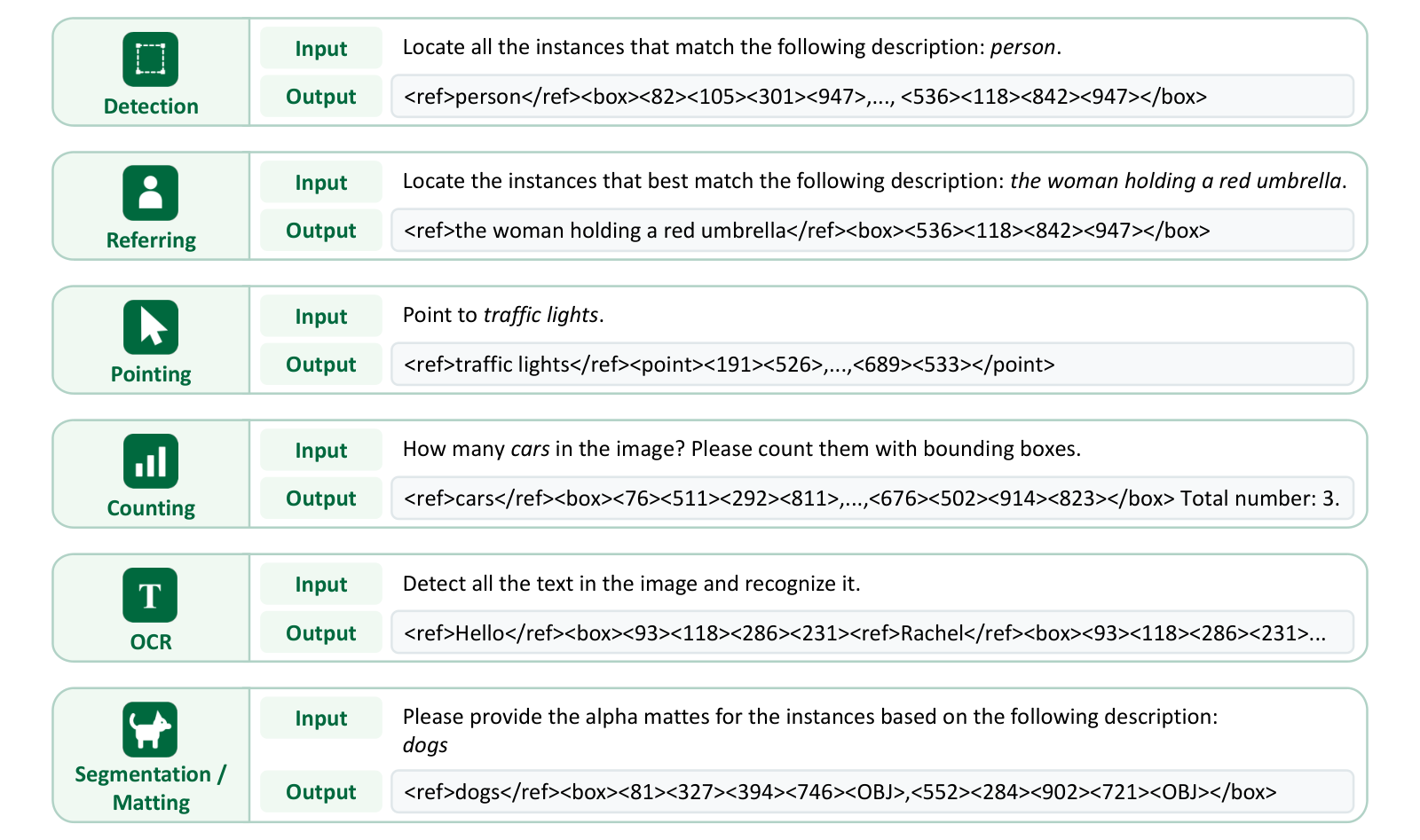
Pixel decoder. A lightweight decoder consumes (i) multi-level ViT features from Qwen3-VL, (ii) the hidden state of each <OBJ> token, and (iii) the predicted box. The decoder builds shared visual features, uses the box to initialize a target query, and iteratively refines it against the visual features to produce a full-resolution mask or alpha matte. Instance identity thus flows cleanly from the autoregressive stream to the dense head via one token embedding per object.
Data engine. The WeVisOne-VL Data Engine (WDE) curates ~100M images and ~3.6B box annotations drawn from GRIT, CC3M, LAION, SA-1B, and task-specific sources.
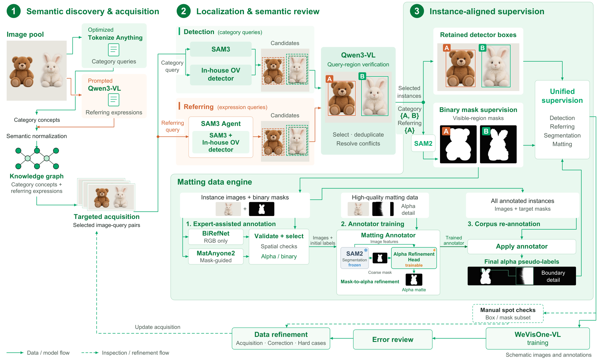
Category concepts (from Tokenize Anything) and compositional referring expressions (generated by Qwen3-VL) are organized in a shared knowledge graph seeded by Wikipedia and WordNet; nodes carry aliases, taxonomic and part–whole relations. Candidate terms are added only when stable visual evidence is retrieved, and acquisition is reprioritized after each training round using model-error review, concept coverage, scale, occlusion, and density.
Training. Three-stage SFT followed by mixed-task RL.
- Stage 1 — Task Alignment. Starting from Qwen3-VL with extended vocabulary, freeze ViT and projector; train the LM on 90M examples for 13K steps covering all tasks, with 16–512 visual tokens/image and 4,096 context. Pixel-task samples use only NTP; the
<OBJ>token learns an initial correspondence to its instance. Dense samples are capped at 50 boxes/points per category to avoid repetitive collapse. - Stage 2 — Resolution and Density Scaling. Unfreeze everything, raise visual tokens to 1,960 and context to 8,192, allow up to 500 boxes/points per response, train on 40M examples for 9K steps.
- Stage 3 — Alternating Token–Pixel Optimization. Warm up the decoder jointly with the SFT-S2 VLM on 250M segmentation samples for 100K steps using \mathcal{L}_{\mathrm{seg}} = 20\mathcal{L}_{\mathrm{focal}} + \mathcal{L}_{\mathrm{dice}}. Then retain only decoder weights and the learned
<OBJ>embedding, attach to the Stage 2 checkpoint, and jointly train 9K steps alternating NTP and pixel losses 1:1: \mathcal{L}_{\mathrm{joint}} = \mathcal{L}_{\mathrm{NTP}} + 10\mathcal{L}_{\mathrm{seg}}. Finally, specialize the decoder for matting on 130M samples for 100K steps with the VLM frozen, using L_1, gradient, and composition losses.
RL then optimizes full-prediction quality rather than per-token likelihood across the mixed task set.
Results
On zero-shot COCO/LVIS and dense Dense200/VisDrone, F1 is reported at IoU 0.5, 0.95, and the 0.5:0.95 mean.
- COCO (zero-shot). WeVisOne-VL-4B reaches 74.0 / 19.5 / 57.1, vs. LocateAnything-3B 70.1 / 19.3 / 54.7 and Rex-Omni-3B 72.0 / 15.9 / 52.9. Qwen3-VL-8B sits at 65.9 / 14.8 / 47.8.
- LVIS (zero-shot). 71.1 / 28.8 / 55.3 for the 4B, versus LocateAnything 62.3 / 31.1 / 50.7 and Qwen3-VL-8B 59.7 / 19.6 / 42.9.
- Dense200. 86.9 / 23.2 / 71.3 for the 4B, +12.6 mean F1 over LocateAnything (58.7) and +13.0 over Rex-Omni (58.3). Qwen3-VL-8B only reaches 13.8 mean F1.
- VisDrone. 68.1 / 3.9 / 44.7 for the 4B, versus LocateAnything 63.0 / 3.2 / 39.9 and GroundingDINO-T 55.2 / 3.9 / 38.5.
The 2B variant already beats both 3B grounding specialists on all four detection sets in mean F1 (55.2 / 53.3 / 61.4 / 40.4). The strong IoU=0.95 numbers indicate the gains are not merely coverage; coordinates land tightly.
Qualitatively, the model recovers dust-obscured elephants missed by baselines, correctly rejects a referring query combining “white shirt and red shorts” when no instance satisfies both, counts pairs of footwear rather than individual shoes, and returns 42 where Rex-Omni returns 537 on a green-ball counting case. On OCR with curved lettering and dense receipts/instruction sheets, more small text is localized and transcribed.
Limitations and open questions
The paper reports leading mean F1 but IoU=0.95 scores (e.g., 19.5 on COCO, 3.9 on VisDrone) are still far below ceiling, so sub-pixel localization — especially for tiny drone-view objects — remains open. Rejection behavior is demonstrated qualitatively; a quantitative false-positive rate on absent-target benchmarks is not surfaced in the excerpts shown. The <OBJ>-based decoder is bottlenecked by a single token per instance, which may limit mask quality for very large or topologically complex objects, and the three-stage curriculum plus 250M-step decoder warm-up is operationally heavy. The training pipeline mixes RL on top of SFT; the specific reward design and its marginal contribution over SFT are not detailed here.
Why this matters
Unifying tokenized box/point outputs with a thin <OBJ>-gated pixel decoder in one autoregressive VLM, and training it at scale with a dedicated data engine, closes much of the gap between generalist VLMs and specialist detectors/segmenters while retaining language-conditioned rejection. It argues that fine-grained perception does not require abandoning next-token prediction — only extending its vocabulary and attaching a cheap dense head.
Source: https://arxiv.org/abs/2610.31329
Deep Search in Real-World Web Environments
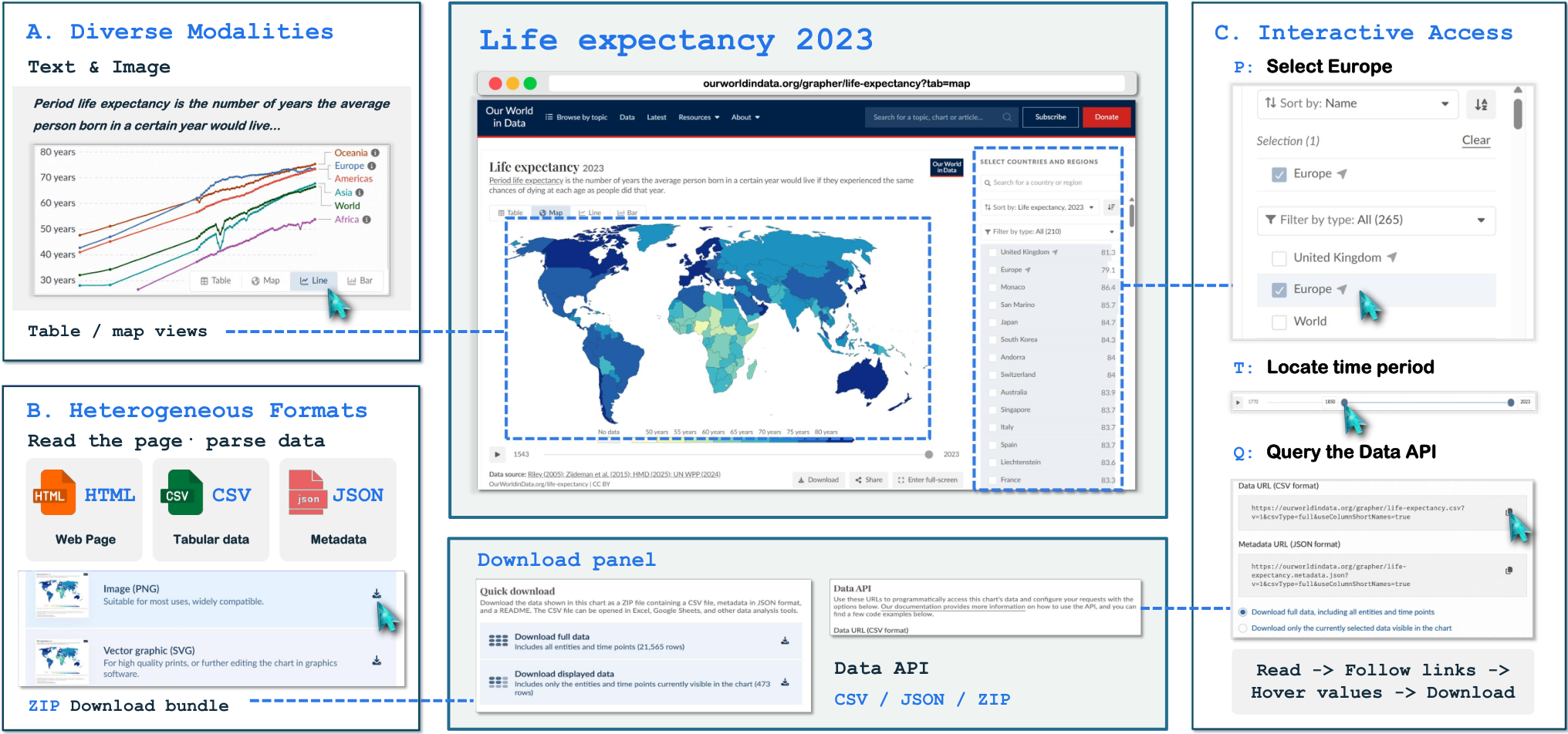
Existing deep-search benchmarks (BrowseComp, GAIA, WebWalker, Humanity’s Last Exam web track) largely treat the Web as a text corpus accessed through search APIs and HTML scraping. This paper argues that real research tasks on the open Web require more: agents must traverse heterogeneous modalities (text, images, audio, video), heterogeneous file formats (HTML, PDF, CSV, JSON, ZIP, Parquet, etc.), and interactive access mechanisms (map viewers, time sliders, API query builders, virtual tours). The authors formalize this as Open-Web Deep Search (OpenDS) and release OpenDS-World, a 200-task benchmark with per-task human-verified evidence chains.
Task formulation
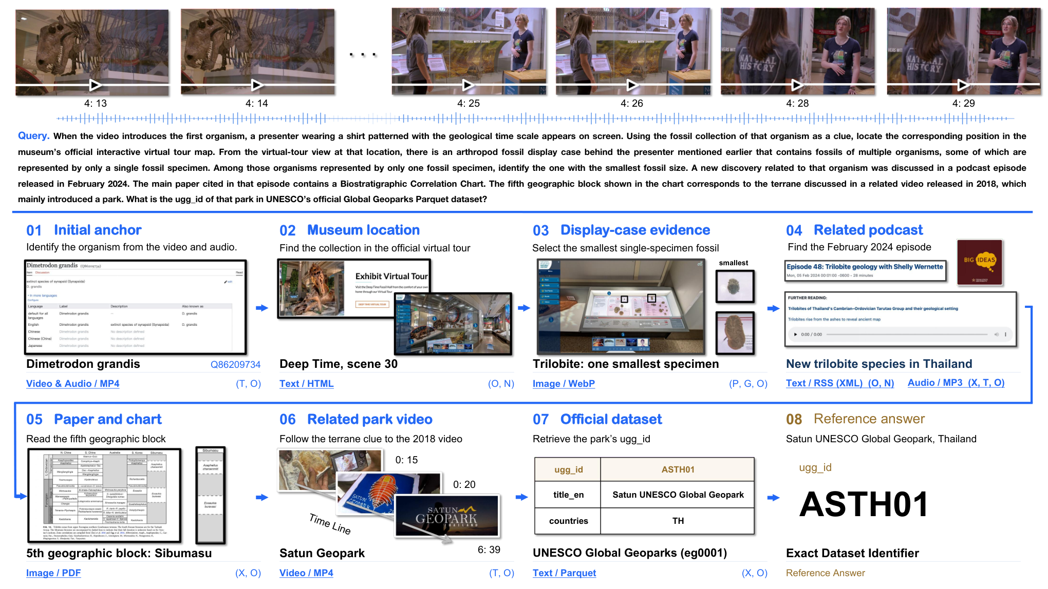
OpenDS is a factual QA task (q, c_0) \mapsto a^\star where q is a question, c_0 an initial clue, and a^\star a unique verifiable answer. Evidence is distributed over an unknown set of sources \{s_1, \dots, s_k\} whose locations and access methods are not revealed. The agent must iteratively plan the next search target, pick an access/processing modality (search, browser interaction, file download/parse, API call), and connect evidence cross-source until it can commit to a^\star. The emphasis is on evidence acquisition rather than only reasoning: an agent that cannot identify a song from an embedded audio clip, navigate a Street View virtual tour, read a specific CSV column, or issue a correct Our World in Data API query cannot finish the task regardless of its reasoning quality.
Figure 2 shows a representative chain mixing audiovisual identification, virtual-tour navigation, document inspection, and structured-data retrieval.
The design is grounded in an observation that a single real-world source already combines three orthogonal properties. The Our World in Data example in Figure 3 illustrates: (A) coexisting modalities (text narrative plus chart images), (B) multiple representations of the same data (HTML, CSV, JSON, ZIP bundle), and (C) interactive controls (region selector, time slider, declarative API). Different combinations of (A)/(B)/(C) yield non-equivalent access strategies even for the same underlying fact.
Benchmark construction
OpenDS-World contains 200 tasks spanning eight domains (culture, daily life, science, economy, history, nature, society, technology). Each task is annotated with an explicit evidence chain, where every entry is tagged with (modality, format, access type). The benchmark covers four modalities, 42 file formats, and seven access types across the 200 tasks (Figure 5). Each entry undergoes independent human verification both for evidence validity and for answer uniqueness, which is critical because many Web facts drift over time or admit near-duplicates on competing sources.
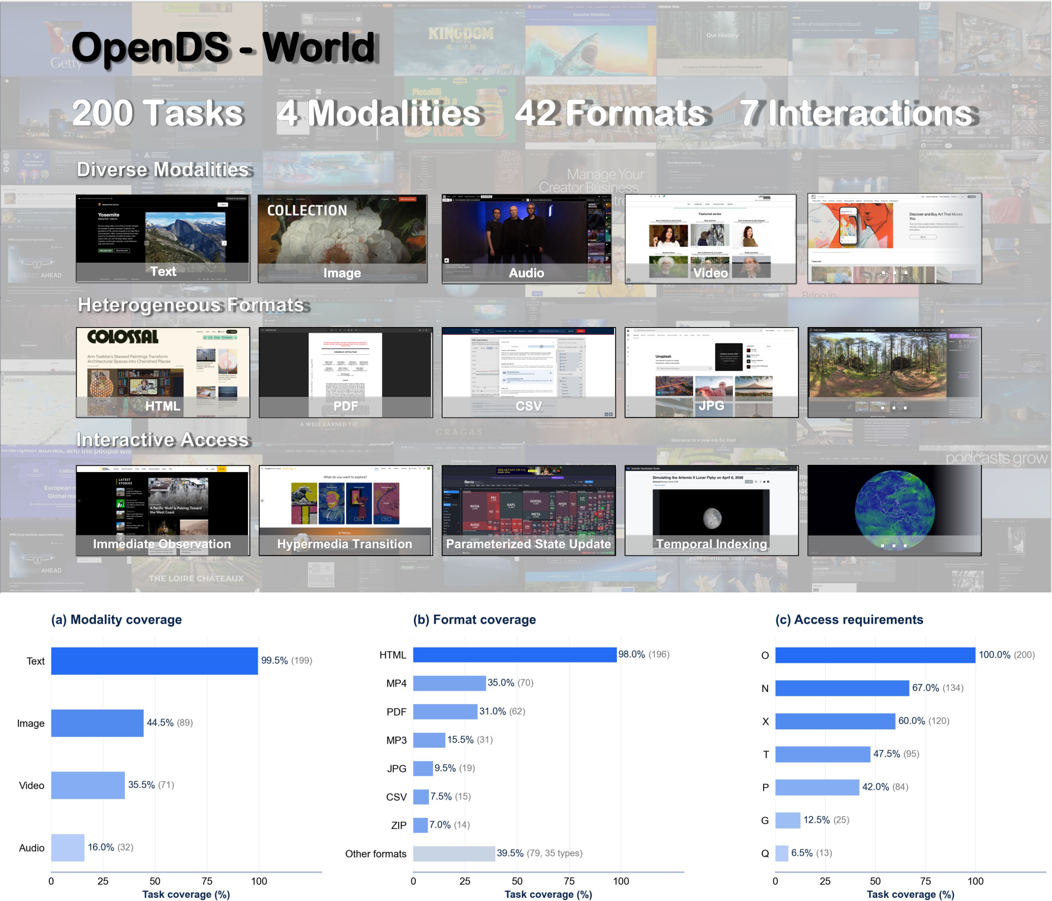
The format coverage (42) is unusually broad for a browsing benchmark — most prior work only hits HTML plus a handful of document types. The access-type dimension (seven categories, including interactive browser manipulation and declarative API queries) is what forces agents beyond search + read loops.
Evaluation protocol
Twelve frontier models are evaluated under identical conditions: same task inputs, same system prompts, same tool environment, same execution budgets. The lineup includes GPT-6 Astra, GPT-5.6 Sol, Claude Opus 5.5, Claude Fable 5.1, Gemini 3.8 Flash, Qwen3.8-Max, Qwen3.8-Flash, DeepSeek-V4.1-Flash, DeepSeek-V4-Pro, Kimi K3, GLM-5.3-Flash, and GLM-5.3. The two-stage prompting splits execution into a research phase (open-ended tool use) and a finalization phase (commit a single answer), with prompts in Appendix C.3. Note: the model names reflect the paper’s near-future release labels; the methodology (fixed tools, fixed budget) is what matters for cross-model comparability.
The sections provided do not expose the headline accuracy table, but the uniform-environment protocol is the right one for isolating model capability from scaffold engineering — a common confound in agent benchmarks where differences in browser harness, retriever, or recursion limit dominate the model signal.
Limitations and open questions
- Live-Web non-stationarity. Evidence pages change, APIs deprecate, and uniqueness of a^\star can degrade over time. The paper relies on human-verified evidence chains at construction time but does not describe a refresh protocol.
- Tool-stack sensitivity. Even with fixed tools, performance on interactive access (virtual tours, dynamic charts) depends heavily on whether the browser harness exposes the needed events; a model that fails on a Street View task may be bottlenecked by the scaffold, not reasoning.
- Multimodal reach. Audio and video identification tasks implicitly test whether the model has access to appropriate perception tools (Shazam-like audio ID, video frame OCR). The benchmark conflates “cannot perceive” with “cannot reason.”
- 200 tasks is small for statistically separating closely matched models; variance across the eight domains is likely substantial.
- The abstract is truncated before reporting the specific accuracies of the 12 models, so the paper’s core empirical claims cannot be verified from the sections provided here.
Why this matters
Browsing benchmarks have converged on a text-centric view of the Web that increasingly diverges from what “doing research online” actually requires: switching modalities, parsing structured data dumps, driving interactive UIs, and composing API queries. OpenDS-World operationalizes those requirements with a modality/format/access taxonomy and human-verified evidence chains, giving a cleaner measurement of whether agent progress is real or artifact of easy retrieval settings.
Source: https://arxiv.org/abs/2610.30181
Editing Images into Reusable Layers via Compositional Edit-Prior Distillation
Instruction-driven image editors produce flat raster outputs, which are convenient for display but destructive for downstream workflows: once an object is pasted or a text block is restyled, the pixel-level provenance of each element is gone. Decomposition pipelines recover layers but typically treat decomposition as a post-hoc step disconnected from the edit itself, so the recovered RGBA stack is not guaranteed to compose back to the intended edit. LayerEditor targets the joint problem — given a source image I^{\mathrm{src}}, an instruction u, and a requested layer count N, produce both an edited canvas \mathcal{D} and an ordered stack \mathcal{S} = \{\mathcal{L}_i = (R_i, A_i)\}_{i=0}^{N-1} whose alpha-over composition \mathcal{C} = \operatorname{Comp}(\mathcal{S}) realizes the same edit while remaining individually manipulable.

In-Context RGB–Alpha Token Modeling
The model is initialized from FireRed-Image-Edit-1.1 and adapted via rank-256 LoRA. The key representational choice is to pack the canvas and all layer fields into a single denoising sequence. At noise level \sigma_t,
Z_t = [z_t^{\mathcal{D}},\, z_t^{R_0}, z_t^{A_0},\, \ldots,\, z_t^{R_{N-1}}, z_t^{A_{N-1}}],
with all fields initialized from Gaussian noise and jointly denoised under shared attention. Field identity and stacking order are encoded through a layer-aware rotary coordinate (s, x, y): source tokens use s=-1, canvas s=0, and layer i gets s=2i+1 (RGB) and s=2i+2 (Alpha). This cleanly supports variable N with a single architecture while preserving spatial correspondence across fields through (x, y). A dedicated Alpha decoder, initialized from the pretrained RGB decoder and trained with opacity plus compositional reconstruction objectives, handles continuous opacity and semitransparent boundaries without disturbing the pretrained RGB pathway.
Compositional Edit-Prior Distillation
Fine-tuning a pretrained editor on layered outputs tends to erode its editing prior. C-EPD counteracts this by using the frozen teacher (the original editor) to supervise both branches of the student: the directly predicted canvas \mathcal{D} and the composition \mathcal{C} obtained by alpha-over-rendering the predicted layers through the Alpha decoder.
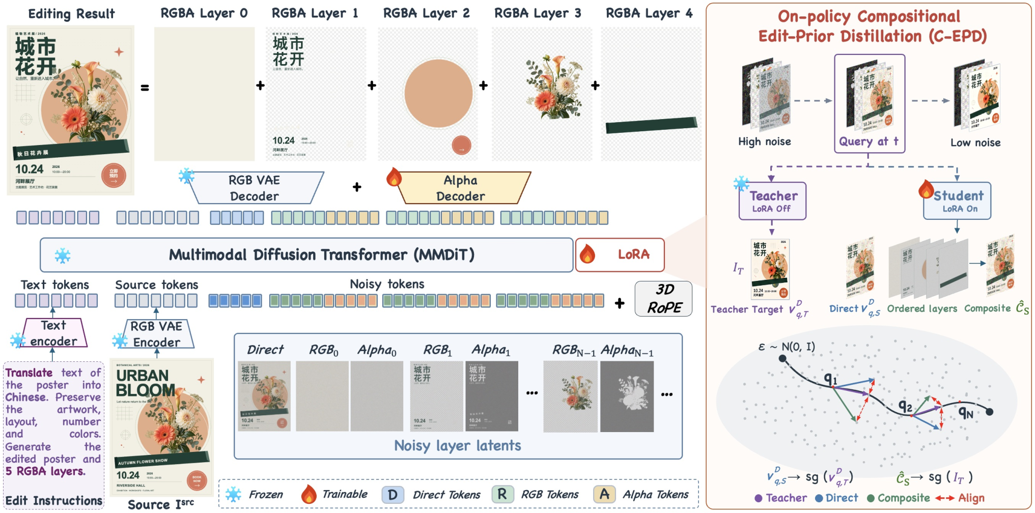
Supervising \mathcal{C} — not just \mathcal{D} — is what ties the layer stack back to the edit distribution: the gradient flows from the teacher’s edit prior through the composition operator into each (R_i, A_i). Training uses two epochs of flow-matching \mathcal{L}_{\mathrm{flow}} followed by joint optimization with C-EPD (AdamW, lr 2 \times 10^{-5}, batch size 64, aspect-preserving within 1024 \times 1024).
LayerEditor-100K
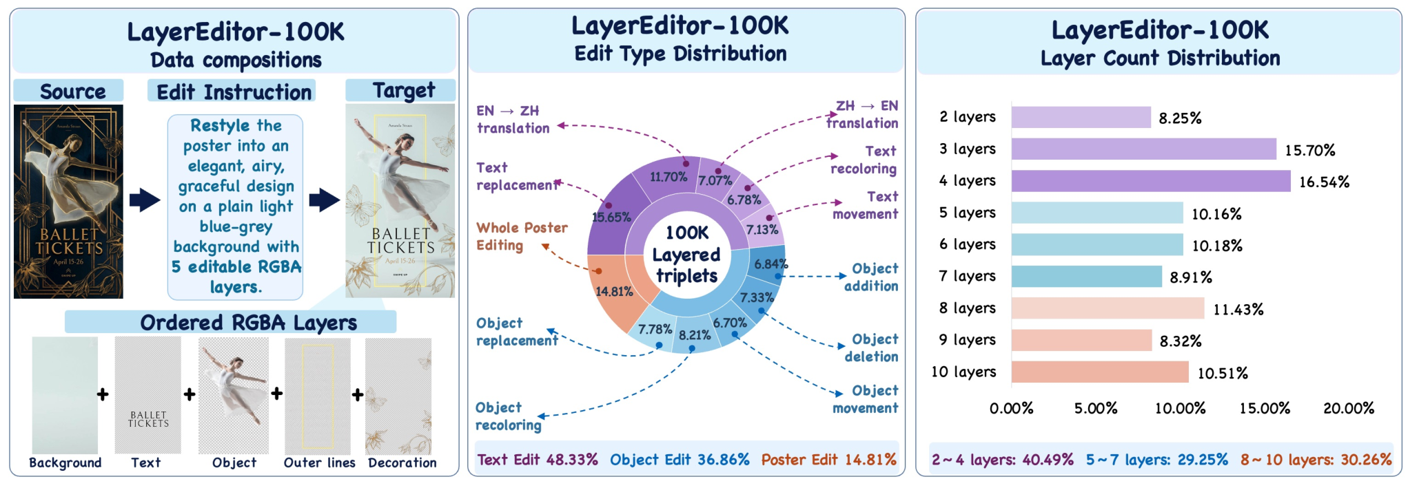
Training data is the other half of the story: paired edits with ordered RGBA ground truth did not exist at scale. LayerEditor-100K provides 100K paired examples with 2–10 layers covering text, object, and poster-level appearance edits.
Results
On Crello-Testset (2,994 documents), LayerEditor dominates every column. For the Direct canvas, SSIM is 0.8530 vs. 0.8586 for Seedream5-Pro (sequential) and 0.7404 for QIL-Edit-SFT, with FID 30.15 vs. 33.04 and 56.85 respectively. The gap widens on the composition: Comp. SSIM 0.8351 vs. 0.7902 (Seedream5-Pro joint) and 0.6343 for FR+QIL-Decomp-FT; Comp. FID 33.86 vs. 55.33 and 57.15. Layer-level fidelity shows the same pattern — RGBA L_1 of 0.0350 (next best 0.0993 from QIL-Edit-SFT, 0.1344 for Seedream5-Pro joint) and Alpha IoU 0.6074 vs. 0.5139 and 0.3171. Rubric scores (1–10) move together: Edit Consistency 6.14, Visual Quality 6.35, Layer Segmentation 6.83, Layer Composition 5.64, Alpha Accuracy 5.05, all above the next-best method by roughly a point.
ScaleEdit-Testset (1,000 documents) replicates this. LayerEditor reaches Comp. SSIM 0.8839 and Comp. FID 39.48 (next-best Comp. FID is 49.37 from FR+QIL-Decomp-FT; Seedream5-Pro joint sits at 59.62), with Alpha IoU 0.6802 vs. 0.6583. Notably, every QIL-based baseline collapses on Alpha Accuracy (1.1–2.2) despite reasonable segmentation scores, suggesting their alpha channels are closer to hard masks than genuine opacity — exactly the failure mode the separate Alpha decoder and compositional supervision target.
Limitations and open questions
The method inherits the base editor’s compositional ceiling: C-EPD propagates the pretrained prior, so systematic failure modes of FireRed-Image-Edit-1.1 should persist. Scaling behavior with N beyond 10 layers is not reported, and the joint sequence grows as 2N+1 fields, making attention cost quadratic in layer count. The ordered back-to-front stack also presupposes an unambiguous depth ordering, which is ill-defined for occluding translucent elements. Finally, rubric-based scores on composites are LLM/human-adjacent and should be read alongside the hard metrics.
Why this matters
Layer-faithful editing — where the composition of the predicted RGBA stack equals the intended edit — is the missing link between generative editors and real design tooling. Distilling the editor’s own prior through the composition operator is a clean way to make decomposition and editing consistent by construction, rather than hoping a separately-trained decomposer agrees with a separately-trained editor.
Source: https://arxiv.org/abs/2610.24738
Deep Fusion Memory: A Chunk-Level Parametric Memory for Large Language Models
Problem
LLMs face a three-way tradeoff when absorbing external knowledge. Continued pretraining risks catastrophic forgetting; inference-time retrieval adds latency, index infrastructure, and context-length pressure; and existing parametric-memory methods (e.g., kNN-LM-style distributions, MLP Memory) require token-level offline retrieval to construct training targets—on the order of one retrieval per token—and typically fuse memory only at the output logit level, which limits how deeply the memory can participate in reasoning. Deep Fusion Memory (DFM) attacks both the construction cost and the shallow-fusion limitation.
Method
DFM has three components trained jointly with the backbone frozen:
Target memory construction (offline). A training sequence is split into non-overlapping chunks X_0, \ldots, X_{J-1} of C=32 tokens. For each chunk X_j with j \geq 1, the preceding chunk X_{j-1} is encoded with a frozen text encoder (Qwen3-Embedding-0.6B) and used to retrieve the top-K=16 neighbors from the Wikipedia datastore. Stacking their frozen embeddings in rank order yields target memory V_j \in \mathbb{R}^{K \times d_m}. Crucially, retrieval is done once per chunk, not per token: 32\times fewer queries and 2048\times fewer retrieved items than token-level schemes using similar K.
Causal memory predictor. A learned predictor maps a pooled embedding of the preceding context to a predicted memory tensor \hat V_j \in \mathbb{R}^{K \times d_m}, supervised by MSE against V_j. Rank-ordered slots give the predictor a stable assignment target. A shared projector then maps \hat V_j into the decoder’s hidden dimension.
Gated cross-attention fusion. At selected decoder layers \{9, 16, 24, 31\} (for the 32-layer Mistral/Qwen backbones), each token hidden state attends to the chunk’s memory slots through an added cross-attention module. A per-head learned gate blends the memory-attention output with the ordinary self-attention path, so the fusion can be modulated or shut off per head.
The joint loss is next-token cross-entropy plus the memory-prediction MSE. Added modules total about 0.75B parameters on the 7B/8B backbones (0.6B on Qwen3-4B); LoRA baselines are matched to this budget. Training uses AdamW at 1\times 10^{-5}, 2048-token sequences, global batch 128, one epoch on 4B Wikipedia tokens. At inference there is no retrieval: the predictor manufactures memory from the running context.
Results
On six QA benchmarks with Mistral-7B-v0.3, DFM reaches an average of substantially above the baselines: NQ 33.57, WebQA 42.47, HotpotQA 29.x (table truncated), with the base model at 13.63 average, RAG at 23.41, xRAG at 24.14, RETRO at 13.73 (essentially no gain over base), CPT at 13.48 (−0.15 vs base, confirming forgetting under full-parameter continued pretraining), LoRA at 15.47, and the strongest parametric baseline MLP Memory at 22.09. The jump from 22.09 (MLP Memory, output-level interpolation) to DFM’s reported scores supports the paper’s central claim that fusing memory into intermediate hidden states beats shallow output-level fusion, even using the same corpus. DFM also matches or exceeds RAG and xRAG without any inference-time retrieval.
The ablations in Section 5 are informative on design robustness:
- Chunk size. Averages of 26.51 / 27.21 / 27.07 for C \in \{16, 32, 64\}. Doubling to 64 halves retrieval queries at a 0.14-point cost; halving to 16 doubles queries with no gain.
- Fusion placement. Spreading four fusion layers across intermediate and late depths [9,16,24,31] yields 27.21, while concentrating at the final layer gives 21.11 and the last four layers [28,29,30,31] give 22.07. A spread-out [2,10,21,31] scores 26.32 (0.89 below default), suggesting that very early layers are not useful insertion points but mid-to-late layers are. Depths of 4, 6, 8 fusion layers lie within 0.13 points, so four is a reasonable default.
- Memory slots. K \in \{2,4,8,16\} give 26.88 / 27.04 / 27.09 / 27.21. Top-2 is within 0.33 of Top-16, indicating that the memory bottleneck is quite narrow and that compute savings from smaller K at the cross-attention are nearly free.
On domain adaptation (Code, Math, Law) with Qwen3-4B/8B-Base, DFM is used as a per-domain adapter against Swallow-Code, Swallow-Math, and DISC-Law-SFT, evaluated on HumanEval/HumanEval+, GSM8K, and LawBench; the paper reports gains while preserving the frozen backbone (specific numbers in Section 4.3 of the paper).
Limitations and open questions
- The target memory is a frozen bag of top-K retrieved embeddings; prediction quality is bounded by the retriever and encoder. The MSE objective treats slots as a rank-ordered set but there is no explicit alignment loss, and the paper does not report how predictor error correlates with downstream accuracy.
- All experiments adapt to a single corpus per task; it is unclear how DFM behaves under corpus updates (one would have to re-train the predictor if the datastore shifts, since there is no inference-time retrieval).
- Added parameter overhead is non-trivial—0.75B on a 7–8B model, roughly 10% expansion—so comparisons to compute-matched LoRA with heavier training (not just one epoch) would sharpen the story.
- Only C=32 with intermediate-to-late fusion is explored seriously; interaction with long contexts (>2048) and streaming inference is not evaluated.
Why this matters
DFM shows that chunk-level parametric memory, fused into hidden states via gated cross-attention, can beat both inference-time RAG and output-level parametric memory while cutting offline retrieval cost by orders of magnitude (32\times fewer queries, 2048\times fewer items). This reframes “memory” from an output-logit interpolation trick into an internal representation that the transformer can actually reason over.
Source: https://arxiv.org/abs/2610.25100
LaLa-World: Scaling Latent World Models with Natural Language Actions
Problem
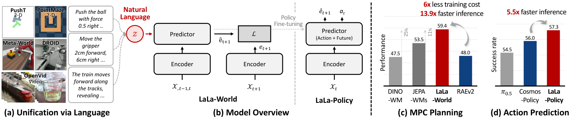
Latent world models (LWMs) in the JEPA family — DINO-WM, JEPA-WMs, and related work — predict future embeddings from past embeddings conditioned on a numerical action vector c_t. Because action spaces differ in dimensionality and physical meaning across robots and simulators, each domain typically requires its own predictor, and ambient video/image data (which has no numerical actions) cannot be pooled in. This fragmentation limits scaling. Video generation models have the opposite situation: they are trained on heterogeneous data via a shared language-conditioned interface, but they operate in pixel space and are expensive. LaLa-World asks whether a JEPA-style latent predictor can inherit the language-conditioned interface of video generators, enabling a single predictor trained jointly on robot control data, simulation data, and generic video.
Method
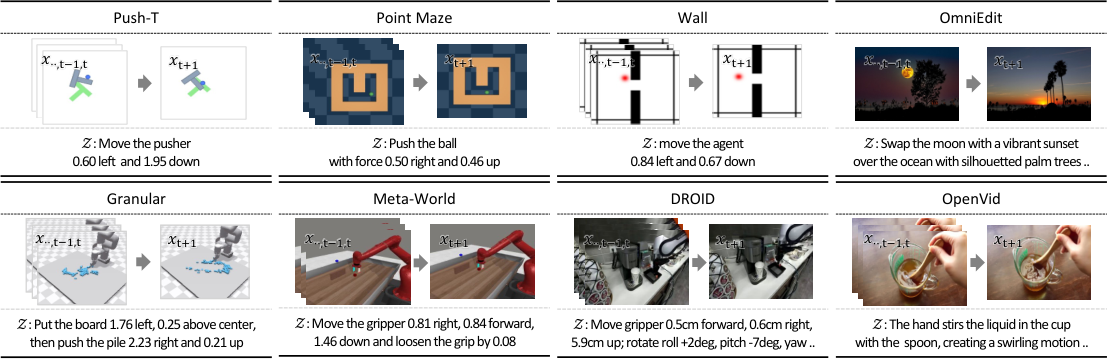
The design has two components. First, a data unification step: every transition (x_t, c_t, x_{t+1}) in simulation and robot datasets is rewritten by template into a language condition z_t that preserves the direction and magnitude of the original numerical action (e.g., end-effector deltas, joint commands). For image/video data without actions, z_t describes the visual change between frames. This gives a single (x_{<t}, z_t, x_{t+1}) format across seven control datasets (Wall, PointMaze, Push-T, MetaWorld, Rope, Granular, DROID) plus image/video corpora.
Second, the predictor P_\phi is built on a language model backbone that ingests the encoded past observations E_\theta(x_{<t}) together with the tokenized language condition z_t and predicts the next latent \hat e_{t+1}. Training uses the standard JEPA objective — regress encoded future E_\theta(x_{t+1}) in representation space — but now with language rather than a numerical vector supplying the action signal. Because the backbone is an LM, it naturally handles variable-form, variable-domain conditions, and benefits from language pretraining to interpret descriptions it has not seen as action phrasings.
Planning
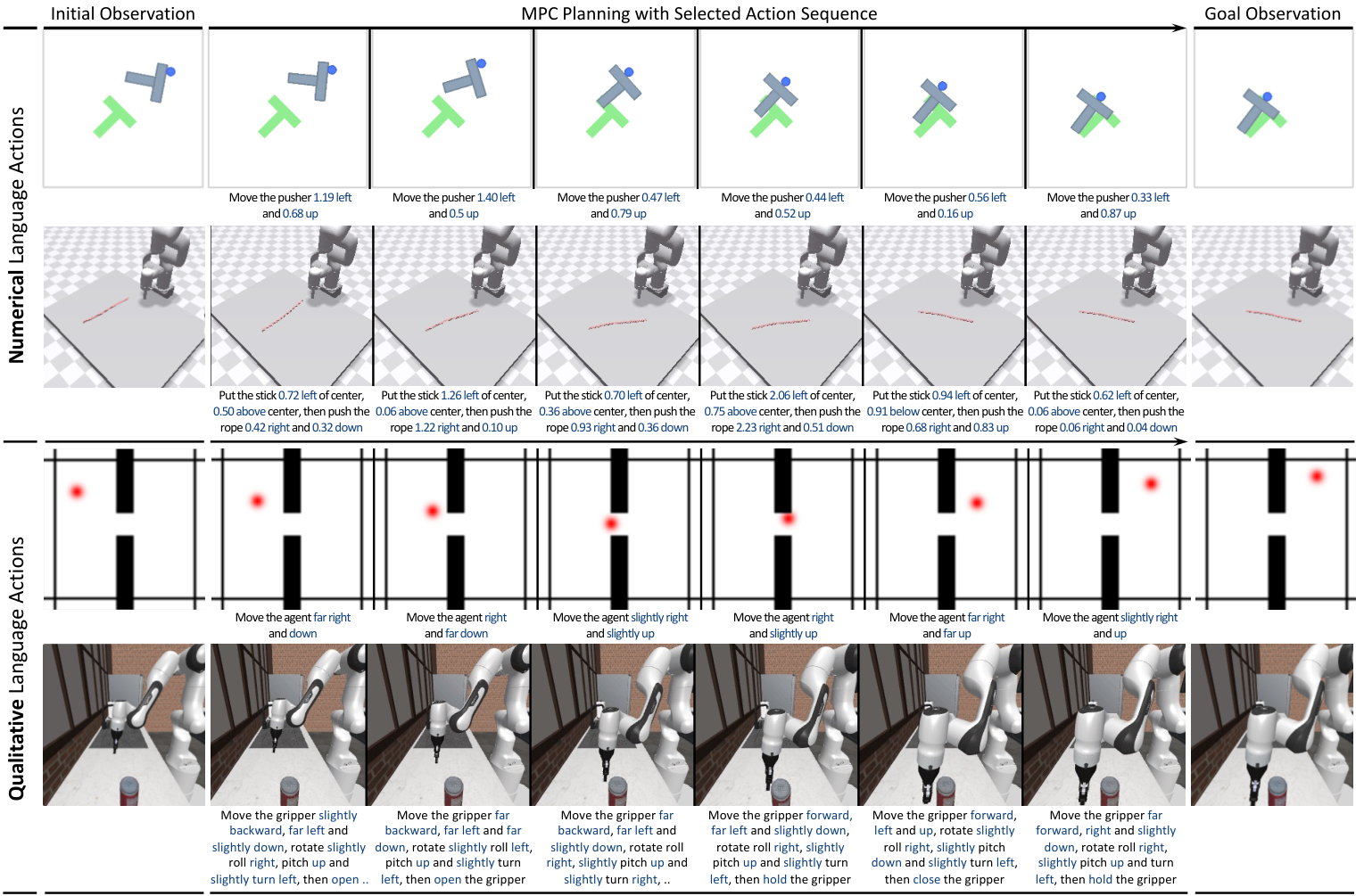
For MPC the authors use CEM over verbalized action candidates. Each candidate action sequence is converted via the training templates into language, rolled out H steps in latent space, and scored by
\mathcal{C} = \|\hat e_{t+H} - e_{\mathrm{goal}}\|^2, \quad e_{\mathrm{goal}} = E_\theta(x_{\mathrm{goal}}).
CEM refits its sampling distribution to the lowest-cost sequences; selected numerical actions (recovered from the templates) are executed, and the loop repeats. Because the interface is shared, a single predictor plans across all seven domains without per-domain heads.
Policy fine-tuning
LaLa-Policy adapts the pretrained predictor following Cosmos Policy’s recipe. Learnable action queries are added to P_\phi alongside the latent-prediction queries. Given (x_t, \ell) with task instruction \ell, the predictor emits a future latent prediction and a sequence of conditioning features h_{t:t+N-1} that drive a diffusion-transformer action head A_\psi (Isaac-GR00T’s architecture):
(\hat e_{t+N}, h_{t:t+N-1}) = P_\phi(E_\theta(x_t), \ell), \hat a_{t:t+N-1} = A_\psi(\epsilon; h_{t:t+N-1}), \quad \epsilon \sim \mathcal{N}(0, I).
The diffusion head preserves multimodality over feasible action chunks.
Results
Across the seven control benchmarks, the single joint LaLa-World predictor achieves higher average MPC planning performance than DINO-WM, JEPA-WMs, and reimplemented IRIS, DreamerV3, and TD-MPC2 world models trained per-domain on the same data (reward-free, no proprioception). Adding image and video data on top of the control mix further improves average planning performance and — importantly — robustness to paraphrased action descriptions, suggesting the LM backbone is actually interpreting the condition rather than memorizing templates. The model also transfers zero-shot to RoboCasa, which was held out of training.
In a matched comparison against a video generation baseline built on RAEv2 (same data, same planning protocol), LaLa-World reaches comparable planning performance with roughly 6\times less compute, which is the main efficiency argument for staying in latent space while adopting the language interface.
Limitations and open questions
The paper’s quantitative claims hinge on CEM-MPC with squared-latent-distance cost, which can be brittle when the encoder E_\theta collapses or when goals are not visually well-specified. Verbalizing candidate actions during CEM adds tokenization overhead that partially offsets the latent-space efficiency win; the exact planning-time cost breakdown vs. the RAEv2 baseline would clarify this. Template-based action verbalization also restricts the “language” to narrow syntactic distributions; the robustness-to-phrasing claim should be stress-tested against adversarial rewordings. Finally, scaling behavior of the LM-backbone predictor as a function of language-condition diversity and video-data volume is not characterized here.
Why this matters
If a single JEPA-style latent predictor can absorb heterogeneous robot, sim, and video data through a language interface and still beat per-domain LWMs at MPC — at a fraction of a video-generator’s compute — then world-model scaling no longer requires either pixel-space generation or per-embodiment action heads. That removes two of the main obstacles to building general-purpose latent world models usable for both planning and policy initialization.
Source: https://arxiv.org/abs/2610.27851
Meta Expert: Cross-Layer Expert Sharing for Storage- and Retrieval-Efficient MoE
Problem
Standard MoE transformers instantiate expert pools independently per layer. Empirically, experts across layers converge to overlapping functions, so a nontrivial fraction of the parameter budget is spent re-learning the same transformations at different depths. Given that MoE scaling is bottlenecked by total parameter count (storage and all-reduce / retrieval cost on expert servers), this redundancy is expensive. The paper asks: can experts be shared across all layers, and does doing so improve information density and training dynamics?
Method
The architectural contrast is a one-line change. In a vanilla “Local Expert” MoE layer l, a layer-private router R_l and expert set \{\phi_e(\cdot;\theta_l^e)\}_{e=0}^{N-1} compute
y_l = \sum_{e\in\mathrm{topk}(R_l,\hat{x}_l)} R_l(\hat{x}_l)_e\,\phi_e(\hat{x}_l;\theta_l^e).
In the “Meta Expert” variant, a single router R and a single pool \{\phi_e(\cdot;\theta^e)\}_{e=0}^{M-1} are shared across every layer:
y_l = \sum_{e\in\mathrm{topk}(R,\hat{x}_l)} R(\hat{x}_l)_e\,\phi_e(\hat{x}_l;\theta^e).
The paper explores two axes of hybridization. The quantitative axis varies the ratio of total and per-layer-activated Meta vs. Local experts, holding both the total expert count and the top-k activation budget fixed to equalize FLOPs. The topological axis varies (a) whether every layer carries both Meta and Local experts, and (b) whether the Meta pool is itself still organized hierarchically (i.e., bands of layers sharing a sub-pool) versus a single global pool. Sweeps are run on a 2B-A0.5B base model; the best configurations are then promoted to a scaling-ladder comparison, where baselines use the training-optimal Vanilla MoE recipe rather than one tuned for shared experts (a conservative choice for the proposed method).
For diagnostics, beyond cross-entropy and downstream accuracy, the authors define an expert-redundancy metric that measures functional overlap between learned experts; this isolates whether reductions in loss are coming from genuine capacity gains or merely from re-parameterization.
Residual-pathway analysis
Section 4 gives the mechanistic argument for why sharing helps beyond parameter dedup. Writing the residual update as
x_{l+1} = x_l + \gamma\, E_{\theta_l}(\hat{x}_l; R_l),
the authors note an asymmetry in Local MoE: the forward pass is strictly causal through layers (content written by layer l can only be read by layers m > l), and even then layer m’s read operator (E_{\theta_m}, R_m) differs from layer l’s write operator (E_{\theta_l}, R_l), so layer l’s contribution is a “frozen” component rather than an addressable one. In the backward pass, the identity residual branch does deliver gradients from deeper layers to \theta_l with unit gain, but this signal is parameter-level, lands only in layer l’s private parameters, and is diluted over the m-l hops by the training signals of all intermediate layers.
Meta Experts collapse this asymmetry: the write and read operators coincide across layers because \theta and R are shared, so content deposited into the residual stream at any layer is directly addressable at every other layer by the same expert index. The paper frames this as a bidirectional residual pathway: shallow layers can functionally “read” from the same expert that deep layers write to, both in the forward pass (shared parameters mean a token at shallow l sees the same transformation that deeper layers rely on) and in training (gradients from deep layers accumulate into the shared \theta as isolated, non-diluted contributions).
Results
With total expert count and activated-expert count fixed, Meta Expert configurations match Vanilla MoE using only 70–80% of the experts. Equivalently, at matched expert count, Meta Expert variants achieve lower cross-entropy and higher downstream task accuracy. The redundancy metric shows that Meta-Expert models have systematically lower overlap among learned expert functions, consistent with the hypothesis that layer-private pools waste capacity learning the same mapping multiple times. These trends persist across the scaling ladder, where baselines retain their own training-optimal configuration.
Limitations and open questions
- The headline 70–80% figure holds under fixed total experts and fixed activated count, which pins FLOPs but not necessarily all-to-all traffic patterns; the paper does not fully report wall-clock or EP communication costs at scale.
- A single global router over a shared pool concentrates routing load; load-balancing dynamics, token-dropping behavior, and router stability at long training horizons are not characterized in the shown sections.
- Hybrid Meta+Local topologies are the best empirical configurations in the sweep, suggesting that pure Meta sharing may lose some layer-specific specialization — the trade-off curve between sharing and specialization is not yet closed-form.
- The residual-pathway argument is qualitative; a quantitative measurement of “addressability” (e.g., causal interventions on expert outputs across layers) would strengthen the claim beyond the loss/accuracy proxies.
Why this matters
Cross-layer expert sharing is one of the few MoE modifications that simultaneously reduces storage, reduces expert-retrieval surface area in distributed inference, and improves per-parameter loss — a rare Pareto move in a design space where most capacity reductions trade off against quality. If the 70–80% expert-reduction result holds at frontier scale, it directly affects how expert-parallel inference systems are provisioned.
Source: https://arxiv.org/abs/2610.27598
Self-Distilling Future Video Representations for World Action Models
Problem
World Action Models (WAMs) repurpose pre-trained video diffusion models (VDMs) as spatiotemporal priors for robot policies. The efficient variant of this architecture — used by DiT4DiT, Fast-WAM, and AGRA — avoids iterative denoising at inference by extracting an intermediate hidden state \mathbf{h} from a single denoising step at \tau_v = 1 (pure Gaussian noise), and feeding \mathbf{h} to a separate diffusion action decoder \pi_\phi(\mathbf{a}_t^{\tau_a}\mid \mathbf{q}_t, \mathbf{h}). The quality of \mathbf{h} — a representation produced from noise, not from a converged denoising trajectory — becomes the bottleneck. The paper asks: can we train the VDM so that its one-shot \mathbf{h} carries the structure a many-step denoised feature would have?
Method: FRED
The authors reinterpret the first layers \mathbf{f}_\theta of the VDM as a future representation generator:
\mathbf{h} = \mathbf{f}_\theta(\bm{\epsilon} \mid \mathbf{o}_t, \mathbf{c}),\quad \bm{\epsilon}\sim\mathcal{N}(\mathbf{0}, \mathbf{I}).
FRED trains \mathbf{h} via self-distillation against a teacher representation \mathbf{h}^\tau computed by the same backbone but on noised ground-truth future frames at a fixed low noise level (\tau = 0.25). The teacher is a momentum EMA of the student, with an inverse-decay warmup. Historical observations (4 past frames plus the current frame) are concatenated as context, which gives the student a temporal prior that a pure-noise input would otherwise lack.
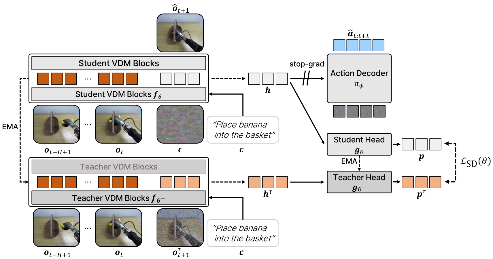
Concretely, features are tapped from a single transformer layer of the VDM — layer 18 (of 19) for Wan2.2-TI2V-5B and layer 24 (of 25) for Wan2.1-I2V-14B — and used for both action-decoder conditioning and the self-distillation target. The self-distillation loss is added to the standard WAM objective with weight \lambda_{\mathrm{SD}} = 0.01:
\mathcal{L} = \mathcal{L}_{\text{VDM}} + \mathcal{L}_{\pi} + \lambda_{\mathrm{SD}}\,\lVert \mathbf{h} - \text{sg}(\mathbf{h}^\tau)\rVert^2.
The action decoder is a 16-layer DiT at 5B scale and a 24-layer DiT at 14B scale. Both L>1 future actions and future observations are predicted jointly within the WAM framework.
The crucial design choices, each ablated:
- Teacher input is noised future observations at fixed \tau = 0.25, not clean frames. Clean-frame targets degrade transfer because the student (starting from pure noise) cannot plausibly reach them.
- Historical observation conditioning — multiple past frames stacked with the current observation — stabilizes the mapping from noise to future.
- Layer choice — late-but-not-final transformer layers carry the strongest predictive signal for action decoding.
Results
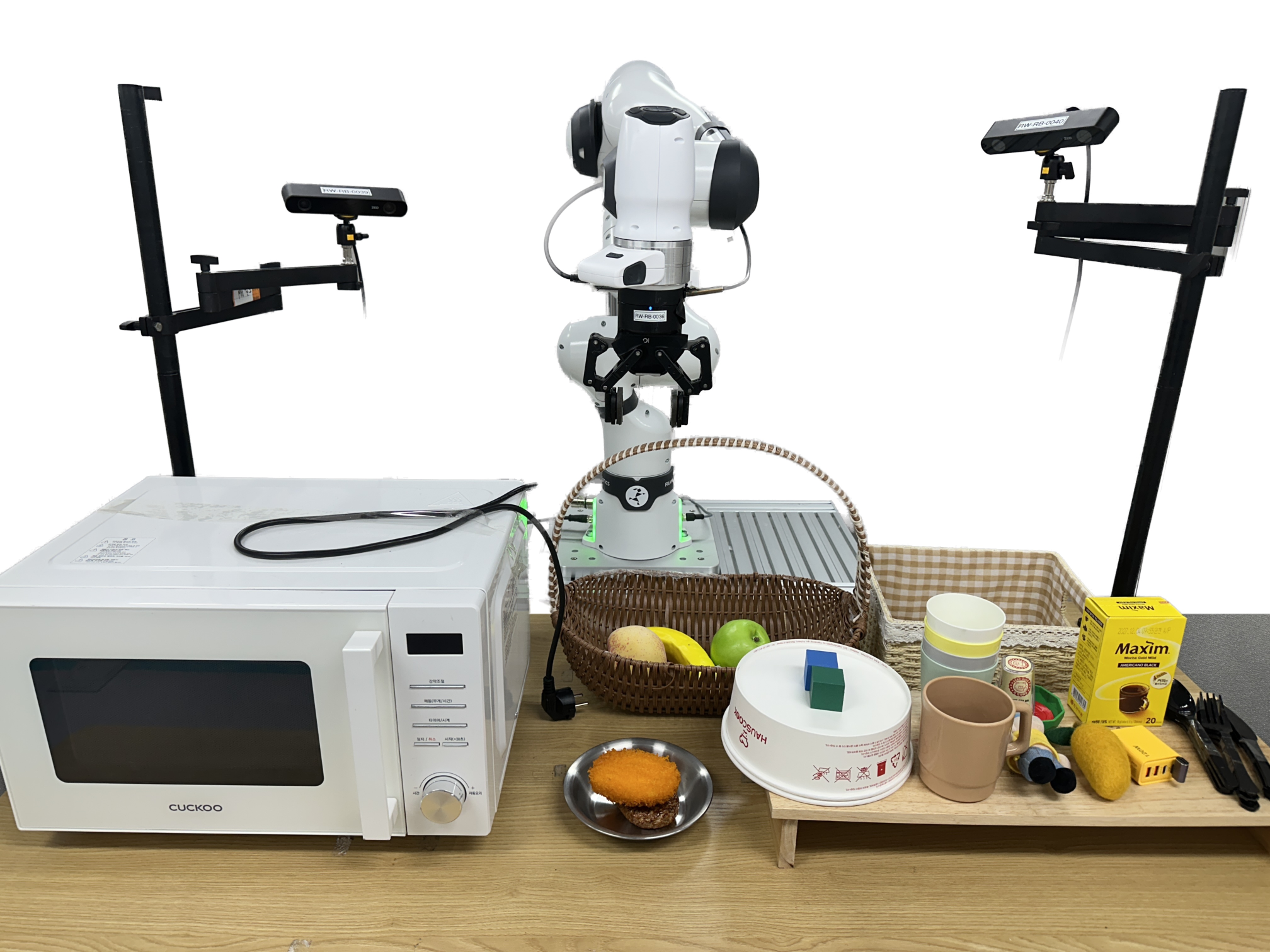
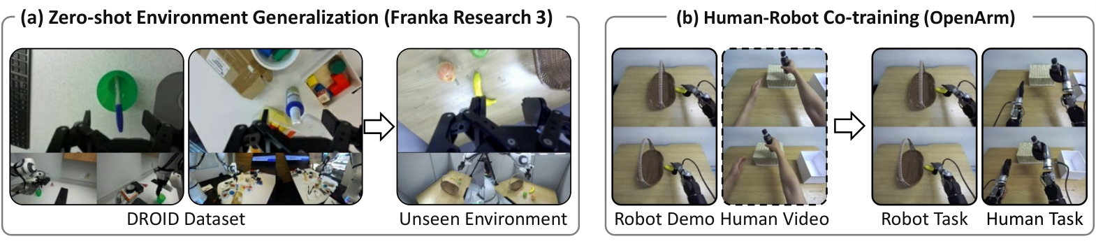
Experiments span two regimes (see Figure 3): zero-shot environment generalization trained on DROID, and human-robot co-training. The DROID evaluation uses a Franka Research 3 with Robotiq 2F-85 and three cameras.
Baselines include single-step WAMs (DiT4DiT, Fast-WAM, AGRA), the multi-step WAM DreamZero, and VLA baselines \pi_{0.5} and GR00T N1.7. Across diverse real-world manipulation tasks, FRED consistently outperforms all competitors at both 5B and 14B backbone scales. The paper additionally reports a positive correlation between representation-quality metrics on \mathbf{h} (Table 4, Figure 4 in the paper) and downstream success rate, supporting the central hypothesis that improving the one-shot \mathbf{h} is the right lever. Human-video co-training yields measurable human-to-robot skill transfer, with FRED benefiting more than the baseline WAMs — consistent with the view that self-distilled \mathbf{h} better absorbs embodiment-agnostic visual priors.
Limitations and open questions
- The feature-extraction layer is a hyperparameter chosen per backbone; the paper does not derive a principled selection rule, and the optimal layer may shift with model scale or domain.
- The teacher noise level \tau = 0.25 is fixed; a curriculum over \tau (bridging student at \tau_v = 1 to teacher at low \tau) is unexplored and could tighten the distillation gap.
- Self-distillation uses an EMA teacher of the same backbone — there is no analysis of representation collapse risk, nor of whether the VDM’s generative loss alone is sufficient to prevent trivial solutions when \lambda_{\mathrm{SD}} is pushed higher.
- The action decoder still relies on a frozen architectural assumption of single-step denoising for the video branch; whether a few extra denoising steps on top of FRED-trained \mathbf{h} would further close the gap to DreamZero-style multi-step WAMs is not quantified.
- Evaluations are real-world and relatively small in task count per table; broader simulation sweeps would help disentangle representation-quality gains from policy-decoder gains.
Why this matters
FRED reframes the efficiency-vs-quality trade-off in WAMs as a representation-learning problem: instead of adding denoising steps, train the one-shot feature to behave like a many-step one via self-distillation against noised future observations. The result is a drop-in training recipe that upgrades the dominant decoupled WAM architecture without changing inference cost, and it provides evidence that future-representation quality — not generative fidelity — is the real target for action-conditioned video priors.
Source: https://arxiv.org/abs/2610.30320
Hacker News Signals
Tsrs: A Port of TypeScript to Rust
Cloudflare is rewriting the TypeScript compiler (tsc) in Rust, targeting a dramatic reduction in type-checking latency for their internal and customer-facing tooling. The project, called tsrs, is not a thin wrapper or a transpiler shim — it is a ground-up reimplementation of TypeScript’s type system semantics in Rust, aiming for full compatibility with the official language specification.
The core motivation is performance: tsc is single-threaded JavaScript, and at Cloudflare’s scale — millions of Workers scripts, continuous CI pipelines — the serial nature of the checker becomes a bottleneck. Rust enables fine-grained parallelism at the module or file level without the GC pauses inherent to the V8 heap. The post details that the initial focus is on the checker pipeline (parsing, binding, type resolution) rather than emit, since emit is comparatively cheap.
Technically, the challenge is faithfully replicating TypeScript’s structural type system, which is notoriously complex: conditional types, mapped types, infer, variance inference, and the interaction between control-flow narrowing and union/intersection types all require careful modeling. TypeScript’s own source is ~300 k lines of TypeScript with significant internal state mutation; a Rust port must decide where to use arenas, where to intern types, and how to handle the recursive type graph without cycles causing borrow-checker issues. The Cloudflare post is candid that they are not attempting 100% compatibility on day one — they are prioritizing the subset of TypeScript most common in Workers scripts.
This is reminiscent of the Ezno and stc efforts, both of which stalled partly on the incompleteness problem. Cloudflare’s advantage is a concrete, constrained workload rather than a general-purpose checker.
Open questions: how they handle declaration file (.d.ts) ingestion for npm packages, and whether the project will converge with Microsoft’s own ongoing performance work on tsc.
Source: https://blog.cloudflare.com/typescript-rust-port/
DeepInfer: High-Performance Inference Framework for DeepSeek Models
DeepSeek released DeepInfer, their first-party inference framework targeting the DeepSeek model family, including the MoE-based DeepSeek-V3 and DeepSeek-R1. The repository positions this as a replacement for generic serving stacks (vLLM, TensorRT-LLM) when running DeepSeek architectures specifically.
The technical differentiators center on MoE routing efficiency. DeepSeek’s models use a fine-grained expert decomposition (256 routed experts, top-8 activation in V3) which creates severe load-imbalance problems under naive batching — different tokens activate different expert subsets, causing irregular memory access patterns and underutilized SMs on GPUs. DeepInfer implements expert-parallel dispatch with a custom all-to-all communication kernel tuned for NVLink and InfiniBand topologies, reducing the expert-routing overhead that dominates latency in multi-GPU configurations.
The framework uses FP8 computation throughout (matching V3’s native training precision), with custom CUDA kernels for the grouped GEMM operations that MoE requires. Attention is handled via a modified FlashAttention kernel with multi-head latent attention (MLA) support, which compresses the KV cache by projecting keys and values into a low-rank latent space before caching — a significant memory saving for long-context inference.
Prefill/decode disaggregation is a first-class design choice: prefill and decode phases run on separate GPU pools, communicating KV state via RDMA. This avoids the prefill-decode interference that plagues unified serving and allows independent scaling of each phase.
The repo ships with benchmark numbers showing substantial throughput improvements over vLLM on DeepSeek-V3 at batch sizes typical of API serving (>1000 tokens/s per H100 node at comparable latency). Independent reproduction of these numbers is still pending from the community.
Limitations: DeepInfer is explicitly scoped to DeepSeek architectures; the abstractions are not designed for generality. Deployment tooling is minimal at initial release.
Source: https://github.com/deepseek-ai/DeepInfer
Google Open-Sources TorchTPU, a Native PyTorch Backend for TPUs
TorchTPU is a PyTorch backend that exposes Google TPUs via the torch.device("tpu") interface without requiring users to touch XLA directly. This is architecturally distinct from the existing PyTorch/XLA (torch_xla) integration, which requires explicit xm.* API calls and a mental model centered on lazy tensor tracing.
The core design uses PyTorch 2.x’s torch.compile and DispatchKey infrastructure. TorchTPU registers as a backend that intercepts ATen operations, lowers them to StableHLO via a custom compiler pass, and dispatches to the TPU runtime. Because it sits at the ATen level rather than the Python frontend level, existing PyTorch code requires fewer modifications — model.to("tpu") and torch.compile(model) are the primary entry points.
The key technical bet is that StableHLO as a stable intermediate representation decouples the PyTorch-to-XLA lowering from TPU firmware updates. Previous torch_xla had coupling between Python-side tracing and XLA’s HLO dialect versioning, which caused fragile version-pinning. StableHLO provides a versioned, serializable IR that can be compiled ahead of time and cached.
Memory management on TPUs differs from CUDA: there is no unified virtual address space between host and device, and buffer aliasing rules are stricter. TorchTPU includes a custom allocator that pre-allocates HBM chunks and manages aliasing for in-place operations explicitly, surfacing errors that XLA would previously silently miscompile.
The HN discussion focuses on whether this replaces torch_xla or complements it. The repo readme is ambiguous, but the architecture suggests eventual convergence, with TorchTPU as the forward-looking path.
Source: https://github.com/google-pytorch/torch_tpu
Using Thousands of AI Agents to Uncover New Leads in Biological Data
OpenAI’s post describes a multi-agent pipeline applied to biological data analysis — specifically re-analysis of existing genomic and proteomic datasets to generate novel hypotheses. The architecture deploys thousands of parallel agent instances, each running a reasoning loop over a scoped data slice, with a coordinator layer aggregating findings and resolving conflicts.
The technical substance centers on agent specialization and communication topology. Rather than homogeneous agents querying a shared database, they use role-differentiated agents: some perform statistical association tests over subsets of a dataset, others retrieve and summarize relevant literature, and a synthesis layer reconciles outputs. The parallelism is embarrassingly parallel at the data-slice level but requires synchronization at the synthesis layer, where conflicting statistical signals must be adjudicated.
A key engineering challenge is preventing agents from hallucinating citations or confabulating p-values. The pipeline enforces that any numerical claim must be derived from a code execution result within a sandboxed Python environment, not generated by the language model token stream directly. This is tool-use grounding at inference time — agents call pandas/scipy/statsmodels and return verified outputs.
The scale claim (thousands of agents) is less about fundamental novelty and more about throughput: the same analysis that a single agent would perform sequentially over days can be parallelized across a fleet, with wall-clock time scaling roughly as O(\log n) for the hierarchical synthesis tree rather than O(n).
Limitations not addressed in the post: inter-agent consistency (do different agents analyzing overlapping data slices agree?), multiple-testing correction across a large agent fleet, and the cost of running thousands of GPT-4-class API calls per analysis pipeline.
Source: https://openai.com/index/scaling-ai-research-for-complex-biological-data/
Using Claude to Reduce the Attack Surface of Code
Anthropic’s research post describes a workflow where Claude is used to systematically identify and eliminate dead code, unused API surface, and unnecessarily exposed interfaces in a codebase. The security premise is straightforward: code that does not exist cannot be exploited.
The technical approach involves prompting Claude with entire modules or file clusters (within context window limits) and asking it to identify: exported symbols with no external callers, branches unreachable under the current call graph, and interface methods that expose more capability than callers require. Claude then proposes refactors that narrow the interface — making public methods private, replacing broad permission grants with least-privilege alternatives, and removing legacy compatibility shims.
What makes this non-trivial is that static analysis tools already exist for dead code detection (e.g., cargo’s unused-import warnings, pyflakes, eslint). The claimed advantage of LLM-assisted analysis is semantic: Claude can reason about whether a public function that is technically called is actually necessary in its current form, or whether a simpler, narrower interface would satisfy all callers. This is a refactoring judgment that requires understanding intent, not just call-graph reachability.
The post includes case studies with concrete metrics: reduction in lines of code, reduction in exported symbol count, and in one case a measurable reduction in CVE-applicable surface area by removing an entire legacy serialization path.
Limitations are significant: the approach requires human review of every proposed change (Claude cannot safely auto-apply refactors to production code), scales poorly to very large codebases without chunking strategies, and cannot reason about dynamic dispatch, reflection, or plugin interfaces without additional context.
Source: https://www.anthropic.com/research/attack-surface-reduction
OpenShell: A Safe, Private Runtime for Fleets of Autonomous AI Agents
NVIDIA’s OpenShell is a sandboxed execution environment designed for running autonomous AI agents at scale, particularly agents that need shell access to accomplish tasks. The core security model isolates each agent in a lightweight container with a controlled syscall surface, mediated by a policy engine that enforces per-agent capability grants.
The architecture has three layers. The first is a container runtime layer built on top of Linux namespaces and seccomp-bpf filters, which restricts the syscalls available to agent processes. The second is a policy layer that translates high-level agent roles (e.g., “this agent may read from /data but not write to /etc”) into seccomp rules and filesystem mount configurations at agent spawn time. The third is an audit layer that logs all agent actions to an append-only store for post-hoc review.
The multi-agent coordination model is notable: agents can communicate via a message-passing bus (not shared memory) that OpenShell brokers, ensuring that a compromised or misbehaving agent cannot directly access another agent’s address space. This is an explicit defense against agent-to-agent prompt injection, where a malicious data artifact consumed by one agent encodes instructions intended to subvert a downstream agent.
GPU access is granted per-agent via NVIDIA’s MPS (Multi-Process Service) with resource quotas, so agents cannot monopolize the GPU or inspect each other’s memory through the GPU side-channel.
The privacy claim relates to data residency: agent workloads can be pinned to specific hardware without data leaving a designated trust boundary, which matters for regulated industries running agents over sensitive data.
Open questions: overhead of the policy evaluation layer at high agent spawn rates, and how the system handles agents that legitimately need to spawn child processes.
Source: https://github.com/NVIDIA/OpenShell
Publish Fake Stats, Get Cited in LLMs
This post is a straightforward empirical demonstration of a training-data poisoning vector. The author created a webpage with fabricated statistics — plausible-sounding numerical claims in a domain with limited authoritative sources — published it, waited for it to be indexed and crawled, and then observed that various LLMs began citing or repeating those statistics in response to relevant queries.
The mechanism is not novel in principle but is practically important. LLMs trained on web crawls do not distinguish between authoritative and fabricated sources at the level of individual numerical claims. A statistic that appears on enough pages — even if all those pages ultimately trace back to a single fabricated origin — acquires the statistical signature of a known fact in the training corpus.
The author’s demonstration is methodologically clean: they chose a niche topic where they could monitor LLM outputs systematically, used a distinctive phrasing that would not appear in legitimate sources, and tracked propagation across model versions and providers. The fabricated statistic propagated into model outputs within a training cycle window.
From a systems perspective, this illustrates a fundamental property of any corpus-trained model: the frequency distribution of a claim in training data is used as a proxy for its truth value, and this proxy is manipulable by a sufficiently motivated actor with the ability to create web-indexed content.
Defenses discussed: retrieval-augmented generation with authoritative source pinning, claim-level provenance tracking in training pipelines, and statistical outlier detection for numerical claims that appear suddenly at high frequency. None of these are fully deployed in production systems at scale.
Source: https://peec.ai/blog/publish-stats-get-cited-the-tactic-that-put-my-data-all-over-the-web
Using LLMs for Confidence Scoring Is a Bad Idea
This post makes a sharp technical argument against using LLM-generated confidence scores as calibrated probabilities, drawing on both empirical evidence and theoretical grounding.
The core problem: when you ask an LLM to output a confidence score (e.g., “rate your certainty 0–100”), the output is not a probability in any meaningful frequentist or Bayesian sense. It is a next-token prediction conditioned on the prompt structure, and the model has been trained to produce plausible-sounding confidence language, not to emit calibrated probability estimates. Post-hoc calibration curves from instruction-tuned models show that verbalized confidence is systematically overconfident on out-of-distribution queries and poorly correlated with actual accuracy across topic domains.
The post distinguishes this from softmax probabilities over the vocabulary at the answer token, which at least have a mathematical grounding (they minimize cross-entropy loss over the training distribution). Verbalized confidence is a layer of natural language abstraction on top of that, introducing additional variance from the prompt framing, the model’s RLHF fine-tuning toward confident-sounding responses, and the lack of any calibration signal during instruction tuning.
A practical example: in a RAG pipeline, using LLM-assigned confidence scores to filter retrieved passages before generation amplifies errors — the model is most confidently wrong on questions where it has seen plausible but incorrect information densely in training data.
The recommended alternatives are ensemble disagreement (variance across multiple samples or model variants), held-out calibration sets with isotonic regression on softmax logits, and for high-stakes settings, conformal prediction intervals which provide coverage guarantees without requiring calibrated probabilities.
The post is concise and cites relevant calibration literature (Guo et al. 2017, Kadavath et al. 2022) without overclaiming. The conclusion is blunt: confidence scores from LLMs are useful as a rough heuristic and should never be treated as probabilities in a decision-theoretic pipeline.
Source: https://rumple.github.io/blog/2026/10/20/asking-llm-for-confidence.html
Noteworthy New Repositories
mw00/project-maya
Project Maya provides a self-hosted inference stack for two large mixture-of-experts models: GLM-5.3-Flash (321B parameters) and DeepSeek-V4.1-Flash-1017 (748B parameters). The core value proposition is private deployment across heterogeneous GPU configurations — from a single consumer card to a 16-GPU cluster — covering both NVIDIA CUDA and AMD ROCm backends on Linux or Windows. The engine handles tensor-parallel and pipeline-parallel dispatch across that range without requiring cloud infrastructure. On top of the inference engine sits an HTTP server exposing both OpenAI-compatible (/v1/chat/completions) and Anthropic-compatible endpoints, so existing tooling drops in unchanged. A built-in dashboard surfaces per-request latency, throughput, and memory pressure. Quantization tooling is bundled, meaning users can compress weights to 4-bit or 8-bit formats locally rather than depending on pre-quantized releases. Running 748B parameters on commodity hardware requires aggressive quantization plus careful KV-cache management; Maya appears to address this by integrating quant-aware loading directly into the engine rather than treating it as a preprocessing step. The main audience is teams that need frontier-scale MoE inference with data-residency constraints or who want to avoid per-token API costs at scale.
Source: https://github.com/mw00/project-maya
pgrundev/pgx
PGX reimplements a lightweight Postgres-compatible runtime in Rust, optimized for the specific workload pattern of AI agent systems: thousands of short-lived, fully isolated database instances within a single process. Standard Postgres imposes per-connection process overhead and is designed for long-lived databases; PGX amortizes that cost by multiplexing many logical databases over a shared Rust runtime with async I/O. Each “database” is a first-class isolated namespace — separate schema, separate storage, no cross-tenant leakage — which maps naturally onto per-user or per-session agent memory stores. The Rust implementation gives deterministic latency without GC pauses, relevant when an agent’s tool call latency budget is tight. Wire protocol compatibility means existing Postgres drivers (psycopg, asyncpg, node-postgres) connect without modification. The use case is agent frameworks that need ephemeral structured storage: spin up a fresh DB per agent run, query it with SQL during execution, discard it after. This avoids the operational complexity of managing a full Postgres cluster while retaining SQL expressiveness over structured agent state. At 391 stars it is early-stage, but the architectural fit for agent workloads is tighter than pointing a full Postgres instance at each session.
Source: https://github.com/pgrundev/pgx
heaven999b/hello-agent-system
A structured curriculum for building production-grade AI agent systems from first principles, delivered as 17 bilingual lessons (English and Mandarin Chinese) with accompanying exercises. The curriculum is organized into layers that mirror real production concerns: tool integration, agent architecture patterns (single-agent, multi-agent, supervisor loops), reliability mechanisms (retries, circuit breakers, fallback chains), security (prompt injection, sandboxing, capability scoping), evaluation frameworks, distributed execution, cost accounting, RAG pipeline construction, and release operations including canary deploys and rollback. Each lesson targets the enterprise deployment context rather than toy demos, which means the exercises involve building pieces — a tool registry, an eval harness, a cost tracker — that compose into a deployable system. The bilingual format is deliberate: both the prose and code comments are maintained in parallel, making it accessible to the large Mandarin-speaking ML engineering community. The “tested exercises” framing implies automated checks against expected behavior, not just open-ended projects. For a CS student or early-career engineer trying to bridge the gap between “I can call the OpenAI API” and “I can deploy an agent system that runs reliably in production,” this provides a more systematic scaffold than most scattered tutorials.
Source: https://github.com/heaven999b/hello-agent-system
onehumanbeing/esp32-iphone-agent
This project wires an AI vision model to a physical iPhone using a $7 ESP32 microcontroller as the hardware bridge. The architecture has two channels: AirPlay is used to stream the iPhone screen to the ESP32 (or an attached receiver) so the vision model can observe display state, and USB HID emulation lets the ESP32 present itself to the iPhone as a keyboard/mouse, issuing taps and swipes. Any OpenAI-compatible vision endpoint (GPT-4o, local LLaVA, etc.) drives the action loop. The constraints are notable for what they avoid: no Mac required means no Xcode or XCUITest dependency; no developer account means no Apple provisioning; no jailbreak means the phone runs stock iOS. The agent loop is essentially: capture screen frame via AirPlay, POST to vision model, parse response into HID events, send via USB. ESP32’s role is purely as a USB HID device and AirPlay sink/relay — the inference happens remotely. Practical applications include automated UI testing on real hardware, accessibility tooling, and physical-world agent benchmarks. The low hardware cost makes it reproducible as a research platform for embodied or GUI agents that need real mobile OS interaction rather than emulators.
Source: https://github.com/onehumanbeing/esp32-iphone-agent
storytold/figcraft
FigCraft is a clean-room reimplementation of collaborative vector-based UI design and prototyping tooling, written entirely in Rust. “Clean-room” signals that it is built from specification and observed behavior rather than derived from any proprietary codebase, which matters for licensing. The technical core is a vector graphics engine, a constraint-based layout system, and a real-time collaborative editing layer — the three hardest components in any Figma-class tool. Implementing this in Rust means the rendering pipeline avoids garbage collection jitter (important for 60fps canvas interaction) and the same codebase can compile to native or to WebAssembly for browser deployment. Collaborative editing at this fidelity requires a CRDT or OT implementation over a document model that represents vector shapes, component hierarchies, and prototype transitions. At 3,188 stars the project has attracted significant attention, likely from teams seeking a self-hostable, auditable alternative to SaaS design tools with data-residency or cost concerns. The open-source model also enables custom plugin APIs, private asset libraries, and on-premise deployment — none of which are straightforward with proprietary tooling.
Source: https://github.com/storytold/figcraft
opengeos/RustGIS
RustGIS is a full-featured geographic information system implemented in pure Rust, positioning itself as a performant open-source alternative to QGIS or GRASS for computational GIS workflows. A pure-Rust implementation means the dependency graph avoids the GDAL/GEOS/PROJ C library stack that underlies most existing GIS tools — those libraries are functional but complex to build and distribute, especially in constrained environments. Rust’s ownership model provides memory safety without a GC, relevant for processing large raster or vector datasets where peak memory is a concern. Core GIS functionality typically includes vector geometry operations (union, intersection, buffer), raster analysis (map algebra, reprojection), coordinate reference system handling, and format I/O (GeoJSON, Shapefile, GeoTIFF). By reimplementing this stack natively, RustGIS can compile to a single static binary, be embedded as a library in other Rust applications, or target WebAssembly for browser-based geospatial tools. The 1,874-star count suggests real interest from the geospatial developer community, which has long dealt with the pain of GDAL build failures and Python environment conflicts. The intersection with AI/ML is direct: spatial feature engineering and geospatial foundation model training both benefit from fast, scriptable GIS operations.
Source: https://github.com/opengeos/RustGIS
Harvil1/codeAgent
CodeAgent is a terminal-resident coding agent that operates over a full repository rather than isolated snippets. The architecture follows the now-standard tool-loop pattern: an LLM planner issues structured tool calls (read file, write file, run command, run tests), observes results, and iterates until a task specification is satisfied. What distinguishes it from minimal wrappers is the repository-understanding layer: before planning, it ingests project structure, infers language/framework context, and builds a representation of the codebase sufficient for multi-file edits. The tool loop is explicitly described as transparent and extensible — meaning tool definitions are inspectable and new tools can be registered without patching core logic. This matters for customization: teams can add project-specific tools (deploy, lint with custom rules, query internal APIs) without forking. Running in the terminal keeps the agent close to the developer’s existing workflow and avoids context-switching to a browser UI. The iterate-until-done loop with test execution as a feedback signal is the key reliability mechanism: rather than generating a patch and stopping, the agent validates its own output and repairs failures. At 1,026 stars it is in the same space as Aider and OpenHands but emphasizes the extensible tool loop as a first-class design goal.
Source: https://github.com/Harvil1/codeAgent
outcrawlai/scout
Scout is an open-source browser agent from Outcrawl, designed for autonomous web interaction and data extraction. The architecture follows the standard browser agent loop: a vision or DOM-parsing module observes page state, a planning LLM selects the next action (click, type, scroll, navigate), and an execution layer drives a real browser via CDP (Chrome DevTools Protocol) or Playwright. Mirroring from Outcrawl’s internal repository means the public version tracks production development rather than a separate community fork. Browser agents are technically hard for several reasons: dynamic pages require waiting for network events before acting, CAPTCHAs and anti-bot measures interrupt naive loops, and mapping high-level task intent to concrete DOM interactions requires either robust element selectors or vision-based coordinate targeting. Scout’s open-source release makes it inspectable for research into agent reliability on web tasks (WebArena-class benchmarks) and adaptable for custom crawling or automation pipelines where commercial browser automation SaaS is too expensive or too opaque. The “by Outcrawl” provenance suggests it is tested against real production scraping workloads rather than being a purely academic implementation.