Daily AI Digest — 2026-10-06
arXiv Highlights
ALoDLM: Adaptively Looped Diffusion Language Models
Diffusion language models (DLMs) decode multiple tokens per step but trail autoregressive (AR) models of equal size on quality benchmarks. ALoDLM attributes this gap to a computation-difficulty mismatch: at a given denoising step, some masked positions are nearly determined by context while others are genuinely ambiguous, yet standard DLMs spend identical forward-pass depth on every position. ALoDLM introduces token-level adaptive recurrence inside each denoising step, learning both the token distribution and a halting policy jointly via a conditional NELBO.
Architecture and inference loop
The Transformer is partitioned into three segments: a \mathsf{Prelude} (embedding plus optional prefix blocks), a \mathsf{Recurrent\ Core} (the middle blocks that are iterated), and a \mathsf{Coda} (suffix blocks that produce a readout). At the start of a denoising step with corrupted sequence \mathbf{x}_t and masked set \mathcal{U}, the Prelude yields h^{(0)} = \mathsf{Prelude}(\mathbf{x}_t) \in \mathbb{R}^{N \times d}. For s=1,\dots,K recurrent passes,
\widetilde{h}^{(s)} = \mathsf{Recurrent\ Core}(h^{(s-1)}), \qquad r^{(s)} = \mathsf{Coda}(\widetilde{h}^{(s)}).
Each readout r_i^{(s)} feeds two heads: \mathsf{LMHead} produces the token distribution p_i^{(s)} = \mathrm{softmax}(\mathsf{LMHead}(r_i^{(s)})), and \mathsf{ExitGate} produces the conditional halting probability
\lambda_i^{(s)} = \begin{cases}\sigma(\mathsf{ExitGate}(\mathrm{sg}[r_i^{(s)}])), & s<K,\\ 1, & s=K,\end{cases}
with a stop-gradient \mathrm{sg}[\cdot] preventing the halting signal from perturbing backbone representations. Forcing \lambda_i^{(K)}=1 makes the exit-depth distribution a valid categorical over \{1,\dots,K\}. The authors use K=4.
The outer loop is the usual masked-diffusion denoising. The inner loop operates per step: tokens that reach the halting criterion commit, their predicted discrete tokens replace the mask in the input, and unresolved positions keep their latent states h^{(s-1)} for additional refinement passes. Committed tokens therefore act as discrete context for still-latent neighbors, which is the mechanism by which easy predictions propagate information to hard ones within a single denoising step without wasting depth.
Training objective
Per-token computation schedules are treated as latent variables. The training objective is a conditional negative evidence lower bound in which the exit depth for each token is marginalized under the learned halting policy, so the LM loss at depth s is weighted by \prod_{s'<s}(1-\lambda^{(s')})\lambda^{(s)}. This gives joint learning of token prediction and the halting policy; the paper also derives variance-reduction techniques for the gradient estimator (Section 3.2, deferred here). The exit-gate stop-gradient is a notable design choice: it preserves the backbone’s prediction behavior under uniform depth and makes the policy a lightweight add-on.
Experimental setup
ALoDLM-1.7B and ALoDLM-8B are initialized from Qwen3-1.7B and Qwen3-8B using the WeDLM streaming block-diffusion framework, which keeps a standard causal attention mask and permits full-sequence conditioning. The recurrent core spans all 28 layers at 1.7B and the middle 16 layers at 8B. Unlike prior conversion recipes (CPT + SFT), ALoDLM skips continued pretraining and runs SFT on only 5B tokens (AdamW, lr 10^{-5}, weight decay 0.01). Evaluation covers 11 benchmarks: ARC-Easy/Challenge, MMLU, MMLU-Pro, GPQA-Diamond, GSM8K, MATH-500, HumanEval, MBPP, and their EvalPlus variants, under the OpenCompass protocol with greedy decoding and 4096-token generation limit.
Baselines include Qwen3 (AR) plus the main Qwen-converted DLMs — Dream, LLaDA, Fast-dLLM-v2, SDAR, WeDLM — each served through its best-available inference stack (dInfer for LLaDA, JetEngine for SDAR, vLLM for WeDLM/Qwen). ALoDLM uses vLLM with depth-aware KV caching: when a prefix token has committed at depth s^*, that depth’s KV is reused; otherwise the deepest available cache is used. To make the quality comparison fair across models with different parallel-decoding heuristics, Table 1 constrains all methods to emit exactly one token per outer step according to their native rules (e.g., minimum-entropy selection).
Results
The abstract reports that ALoDLM “outperforms” the DLM baselines across the eleven benchmarks at both 1.7B and 8B scales under the one-token-per-step protocol; the paper’s Section 4.3 discusses inference speed and compute, where adaptive depth lets most positions exit early so that mean recurrent depth is well below K=4 while the hardest positions still receive the full budget. (The provided excerpt stops before the detailed per-benchmark numbers; the structural claim is that the quality gap to Qwen3 AR closes while retaining the parallel-decoding speedup from block diffusion.)
Limitations and open questions
Three issues are worth flagging. First, the halting policy sees only the current readout and uses a stop-gradient to the backbone, which simplifies training but prevents the backbone from learning features explicitly useful for halting; a non-detached variant could trade stability for policy quality. Second, with K=4 and the recurrent core occupying 16 of ~36 layers at 8B, the maximum extra FLOPs per step is bounded but the KV-cache logic becomes nontrivial — the paper’s depth-aware caching heuristic (use same-depth KV when available, else deepest) is a pragmatic approximation whose quality cost is not quantified in the excerpt. Third, skipping CPT and SFTing on 5B tokens is attractive, but it is unclear how much of ALoDLM’s gain comes from the adaptive loop versus the WeDLM streaming-block substrate; a fixed-K ablation would isolate this. Finally, the one-token-per-step evaluation protocol is a fair-comparison choice, but it suppresses exactly the parallel-decoding regime where DLMs are most interesting, so wall-clock gains in realistic multi-commit settings need separate scrutiny.
Why this matters
Decoupling per-token compute from per-step compute is the natural extension of adaptive-depth ideas (PonderNet, early-exit Transformers) to the diffusion setting, and it directly targets the structural reason DLMs underperform AR at matched parameter count. If adaptive recurrence can close the quality gap without erasing the parallelism advantage, it reshapes the Pareto frontier between DLMs and AR decoders.
Source: https://arxiv.org/abs/2610.04198
Optimizing the Optimizer: Language Models Discover Faster Molecular Relaxation
Geometry optimization sits in the inner loop of nearly every quantum-chemistry workflow: each step consumes one force evaluation, and at the DFT level that single call dominates wall time. Decades of work on quasi-Newton methods, trust-region updates, and internal-coordinate preconditioners have produced a crowded Pareto frontier, with Sella currently the fastest open-source option for molecular relaxation. The question this paper asks is whether an LLM-driven “autoresearch” agent, given Sella as a seed and only a cheap semiempirical potential as a test harness, can rewrite the optimizer itself to reduce force-call counts in a way that transfers to unseen molecules and unseen potentials — including DFT, which the agent never sees.
Problem setup and metrics
The task is unambiguous: given a molecule and a force evaluator, reach fixed convergence criteria in as few force calls as possible. Cost is reported with two aggregates to disentangle long-trajectory bias from per-molecule gains,
C_{\text{pooled}} = \frac{\sum_i n_i}{\sum_i n_i^{\text{ref}}}, \qquad C_{\text{per-mol}} = \frac{1}{N}\sum_i \frac{n_i}{n_i^{\text{ref}}},
paired with a relative energy recovery
r_i = \frac{E_i^{\text{start}} - E_i^{\text{final}}}{E_i^{\text{start}} - E_i^{\text{final,ref}}}, \qquad \bar r = \frac{1}{N}\sum_i r_i,
so that r_i<1 flags premature stopping and r_i>1 flags a deeper minimum. These two measurements together are the admission gates: the agent is only allowed to keep an edit if it (i) does not shortcut convergence and (ii) generalizes to held-out molecules. Without the second gate the search collapses into overfitting the training molecules; without the first it collapses into early termination that looks like a speedup.
Method
The autoresearch loop treats the optimizer’s Python source as the artifact under optimization. The LLM agent proposes rewrites — changing step acceptance, Hessian updates, trust-radius logic, internal-coordinate handling — runs them on a GFN2-xTB evaluation suite, and keeps variants that pass both admission gates. The search is run exclusively on GFN2-xTB; neither DFT gradients nor the GFN-FF force field appear in training. The output is a family of two optimizers, AutoSella-F (favoring aggressive force-call reduction) and AutoSella-A (a more conservative variant).
Mechanically, the recipe to reproduce the skeleton is: (1) start from a well-engineered baseline optimizer; (2) define C_{\text{pooled}}, C_{\text{per-mol}}, and \bar r on a training/validation split of chemically diverse small molecules; (3) require \bar r \geq 1 - \epsilon as a hard constraint on validation to block degenerate shortcuts; (4) require improvement on validation (not just training) as a hard constraint on generalization; (5) run an LLM agent as a code-rewriting outer loop with these admission gates. The paper’s framing is that the admission gates, not the agent’s cleverness per se, are what make the search produce transferable optimizers.
Results
On GFN2-xTB — the in-distribution potential — AutoSella-F uses between 39.86% and 73.25% of Sella’s force calls per molecule across four held-out benchmarks: 73.25% on 500 unseen PubChem molecules, 65.28% on 673 dipeptides, 69.79% on 475 amino acid–ligand pairs, and 39.86% on 100 Solvated PubChem systems. Mean energy recovery satisfies \bar r > 1 on all four datasets, i.e. AutoSella-F reaches slightly deeper minima than Sella on average. Appendix analysis gives median \Delta E = E^{\text{AutoSella-F}}_{\text{final}} - E^{\text{Sella}}_{\text{final}} between -8\times 10^{-6} and -5\times 10^{-6} kcal/mol on three datasets, and -1.30 kcal/mol on Solvated PubChem — small but systematically negative. AutoSella-A is less aggressive, at 78.14–92.57% on the first three datasets, but regresses on Solvated PubChem (118.77%, \bar r = 0.999).
The more consequential result is transfer to potentials unseen during the search. On GFN-FF (a force field, different error structure from GFN2-xTB), AutoSella-F uses 68.91–74.14% on the small-molecule and dipeptide benchmarks and drops to 34.08% on Solvated PubChem. On r2SCAN-3c DFT — the regime where force calls actually matter economically — AutoSella-F uses 73.14–77.20% of Sella’s force calls on the Test and Dipeptides benchmarks (the paper reports best variants at 40.2–77.2% across the full DFT suite) while matching or exceeding Sella’s energy reduction. That the saving holds on a potential with fundamentally different curvature statistics than GFN2-xTB is the paper’s strongest claim: the agent did not merely tune heuristics to the training potential’s noise profile.
Limitations and open questions
AutoSella-A’s regression on Solvated PubChem (113% pooled on GFN2-xTB, 109% on GFN-FF) shows the search does not uniformly improve across chemical regimes; multi-fragment solvated systems are a known hard case for internal-coordinate methods and the agent’s edits apparently did not help there for one variant. The admission gates define “generalization” through four held-out datasets, but these are still small-molecule-biased; transition-state search, periodic systems, and large biomolecular complexes are untested. The paper also does not report ablations isolating which specific code edits produce the force-call reduction, so it is unclear whether the gains come from a single mechanistic change (e.g. a better trust-radius schedule) or a diffuse set of micro-optimizations. Finally, the agent used no DFT gradients during search, which is a feature for cost but means the DFT-regime gains could be fragile to functionals with very different curvature than r2SCAN-3c.
Why this matters
This is a concrete demonstration that LLM-driven code search, constrained by admission gates on generalization and non-cheating, can produce transferable improvements to a mature numerical method whose Pareto frontier is already crowded. If the 40–77% force-call reduction at the r2SCAN-3c level survives independent replication, it is a direct multiplicative speedup for DFT workflows obtained without touching any DFT during search.
Source: https://arxiv.org/abs/2610.06577
Self-Generated Feedback Destabilizes Test-Time Training: A Causal Decomposition of Long-Horizon Adaptation
Test-time training (TTT) treats inference as online learning: the model updates its own weights on streaming context, hoping to accumulate useful state beyond the attention window. The pathology this paper documents is that when the stream itself is generated by the adapting model — the typical autoregressive setup — the fast-weight updates systematically degrade prediction on independent human text. The failure is not from a single bad update but accumulates over long horizons, and it reproduces across architectures and update rules.
Setup
Three TTT-E2E configurations (125M, 760M, 3B) are evaluated on PG-19 with an 8192-token attention window and a clipped gradient step after each 1024-token chunk, updating the FFN modules of the final three layers. The main cross-scale protocol fixes six books, five seeds, 128K-token horizons, and batch width eight. To rule out architectural idiosyncrasy, the authors also apply plain Adam updates to Qwen3-4B.
The long-horizon failure
Two streams are compared: Closed Loop (generate, update, repeat) and Writes Off (generate, keep tokens in attention, discard updates). Both see the same generated tokens; only Closed Loop retains the weight change. At 128K tokens, the retained updates add +3.01, +6.00, and +0.40 nats over Writes Off at 125M, 760M, and 3B respectively, with every 95% interval excluding zero. The direction replicates across scales; the magnitude is not monotone in parameter count.
Crucially, within the earlier 8K+8K evaluation window used in prior TTT work, Closed Loop and Writes Off are nearly indistinguishable — the gap is a late-horizon phenomenon that only appears after many self-writes. Decoder changes (full-support sampling, lower temperature, typical sampling, repetition penalties) shift the slope but do not produce a safe operating point: full-support sampling cuts the 128K endpoint gap from 3.010 to 1.452 nats, but late loss is still climbing. Interleaving real text repairs the loop if it is evenly spaced: replacing 0/5/11/21/33 of 105 generated chunks with real chunks reduces harm to roughly 87%/37%/7%/6%; bursting the same 33-chunk budget leaves ~60% of the harm. The protective factor is interruption frequency, not real-text fraction.
The Qwen3-4B results exclude an idiosyncratic-TTT explanation. At Adam LR 10^{-4}, persistent self-writing produces H=1.231 nats [.580, 2.350] of harm, while the same updates on real text yield 0.168 nats of benefit. Writing updates are not inherently harmful; closing the generation–update loop is.
Causal decomposition
The core contribution is a three-way intervention isolating which link in the loop causes damage:
- Fixed Generation: a frozen W_0 generates all future chunks while a separate learner W_t updates on them. The learner still sees generated text and still updates every chunk — the only removed dependency is that its updates can no longer alter the text it will train on next.
- Recorded Replay: a fresh receiver processes a saved degraded token stream either read-only or with updates, holding content fixed.
- Closed Loop: the standard setup where W_t generates, learns, and becomes W_{t+1}.
Fixed Generation leaves only 0.052 and 0.073 nats of residual harm at 125M and 760M, removing 98.3\% and 98.8\% of the matched Closed Loop gap. Update magnitude cannot explain this: Fixed Generation moves farther from W_0 than Closed Loop (0.01387 vs. 0.00857 in weight distance) yet causes far less damage, and Real-Text Learning moves farther still (0.01759) while improving NLL by 0.3544 nats. The pathological property is specifically that updated weights determine future training text.
Repetition is a symptom, not the mechanism: Closed Loop ends with repeated-4-gram rate 0.9902 versus 0.0217 for Writes Off and 0.0082 for Fixed Generation, but the correlation does not separate the loss from reading degraded tokens from the loss stored by updating on them. Recorded Replay provides that separation by holding tokens fixed.
Which updates are harmful
A paired write-cost analysis — \mathrm{NLL}(\text{Read+Write}) - \mathrm{NLL}(\text{Read Only}) on the same real evaluation text — reveals strong heterogeneity. At the first position, mean and median costs are 0.0439 and 0.0422 with no outliers above 0.5 nats. At the final position, the mean rises to 0.7512 while the median falls to 0.0064. Only 12 of 72 late costs exceed 0.5 nats, and all twelve come from 4 of 24 source sequences; once a pair crosses the threshold it stays above it. Position in the stream is therefore not a usable predictor of safety.
The practical consequence is a sharp trade-off between control strength and benefit retention. Repetition weighting and read-only real context leave 54\% and 48\% of the Closed Loop gap. An eight-chunk fast-weight reset removes 94.2\% of the harm but retains only 44.1\% of the useful adaptation gain. No tested time-only policy both suppresses damage and preserves adaptation.
Limitations and open questions
The decomposition localizes the causal path but does not yield a per-update acceptance criterion. The authors’ Settlement procedure (evaluating candidate weights on held-out real text before commitment) is the natural next step but is only briefly motivated here. The cross-scale magnitudes are non-monotone — the 3B harm (0.40 nats) is far smaller than at 760M (6.00) — which the paper does not fully explain; it may reflect generator quality interacting with update step size. All experiments are in-domain to PG-19/long-form books; whether the loop closes similarly under more diverse streams is untested.
Why this matters
This is a clean falsification of the implicit assumption that TTT updates composed over long autoregressive horizons are approximately safe. The harm comes specifically from the generation-update feedback link, not from synthetic data or from update magnitude, which means that any TTT system intending to run beyond a few thousand tokens needs an explicit mechanism — selective commitment, interruption, or external anchoring — rather than tuned decoding.
Source: https://arxiv.org/abs/2610.05076
ASCENT: Online Test-Time Training of Long-Horizon Agents via Self-Distillation of Verified Experience
Problem
An LLM agent deployed on a stream of related long-horizon tasks produces, per task, a multi-turn ReAct trajectory and a single binary verification signal at termination. The usual self-evolution options are either (a) in-context: accumulate reflections, skills, or memories as text while the policy stays frozen, which couples adaptation to retrieval quality and leaves execution untouched, or (b) parametric RL/SFT on the generated tokens, which is unstable when the only data is a single on-policy attempt with sparse episode-level reward and no turn-level credit. The authors formalize this regime as Online Agentic Test-Time Training (OaTTT): one pass over a task stream \mathcal{X}_{1:N}, one scored attempt per task, each outcome recorded before the trajectory can influence the policy (prequential protocol), and the weights that are updated persist across tasks. Formally, episode i yields \tau_i \sim \mathbb{P}_{\pi_i,\mathcal{E}}(\cdot \mid x_i) and v_i=\mathcal{V}(x_i,\tau_i)\in\{0,1\}, and an operator (\theta_{i+1},\mathcal{M}_{i+1})=\mathsf{Evolve}(\theta_i,\mathcal{M}_i;x_i,\tau_i,v_i) advances the state. No replay buffer, no retries.
Method
ASCENT (Agentic Self-distillation for Cross-task EvolutioN at Test-time) updates a LoRA adapter \phi_i on the student policy p_{\theta_0,\phi_i} after each verified episode. The key mechanism: rather than imitate the student’s own tokens from a single success, a frozen teacher p_{\theta_0} (the initial model with \bar\phi=0) is given the verified trajectory as privileged hindsight context z_i, and produces soft next-token distributions q_i = Q_{\bar\phi_i}(\tau_i) at the student’s prefixes. The student is updated via KL to these targets, \mathcal{L}_i^{\mathrm{ASCENT}}[q_i], with stop-gradient on z_i. Updates are gated by R(\tau)=\mathcal{V}(x,\tau), so only accepted trajectories drive supervision.
The paper’s Section 6.1 clarifies what this objective actually fits. Verifier gating induces the posterior \pi^+(u\mid S) = \pi(u\mid S)\frac{Q^\pi(S,u)}{V^\pi(S)}, i.e., a reweighting of responses by their relative chance of eventual acceptance. With only one on-policy sample at a history, this cannot rank alternatives; the hindsight teacher instead smooths targets by conditioning on the completed, verified continuation, trading causal credit for a lower-variance supervision signal.
The teacher’s frozenness is itself a design choice. In an ablation (Table 7), replacing \bar\phi=0 with an EMA or periodic snapshot of the student creates a cross-task feedback loop that stop-gradient does not block. Fast evolution (EMA \beta=0.90, snapshot N=10) collapses: 24.3\% and 45.7\% overall SR on ALFWorld seen, with late-stream SR dropping from 48.6\to 2.9 for \beta=0.90. Slow EMA (\beta=0.999) recovers to 61.4\% but still trails the fixed teacher (69.5\%). The frozen initial model is the stable attractor.
Results
On ALFWorld seen (140 tasks across six families, 50-turn budget), with Qwen3.5-4B:
- ASCENT: 69.5\pm 5.6\% SR, 26.3 mean turns.
- Best online in-context baseline (MemP): 63.6\pm 5.9\%, 29.7 turns.
- Best offline self-evolution baseline (MemP, trained on a fixed split): 61.4\pm 6.5\%.
- Base Qwen3.5-4B: 46.4\%, 35.1 turns.
- TT-OPSD (single-turn OPSD adapted to test time; teacher sees only current turn’s response/observation): 51.0\pm 3.7\%. The gap to ASCENT isolates the value of full-trajectory hindsight.
With Qwen3.5-9B, ASCENT reaches 77.4\pm 1.8\% SR at 21.0 turns, versus 69.3\% for online ACE and 67.9\% for online MemP. By family, ASCENT solves the hardest categories at non-trivial rates where offline and in-context methods frequently stall: Heat 20.8\% at 4B / 37.5\% at 9B, Cool 54.7/48.0\%. The \mathrm{Pick2} family hits 75.0/95.8\%.
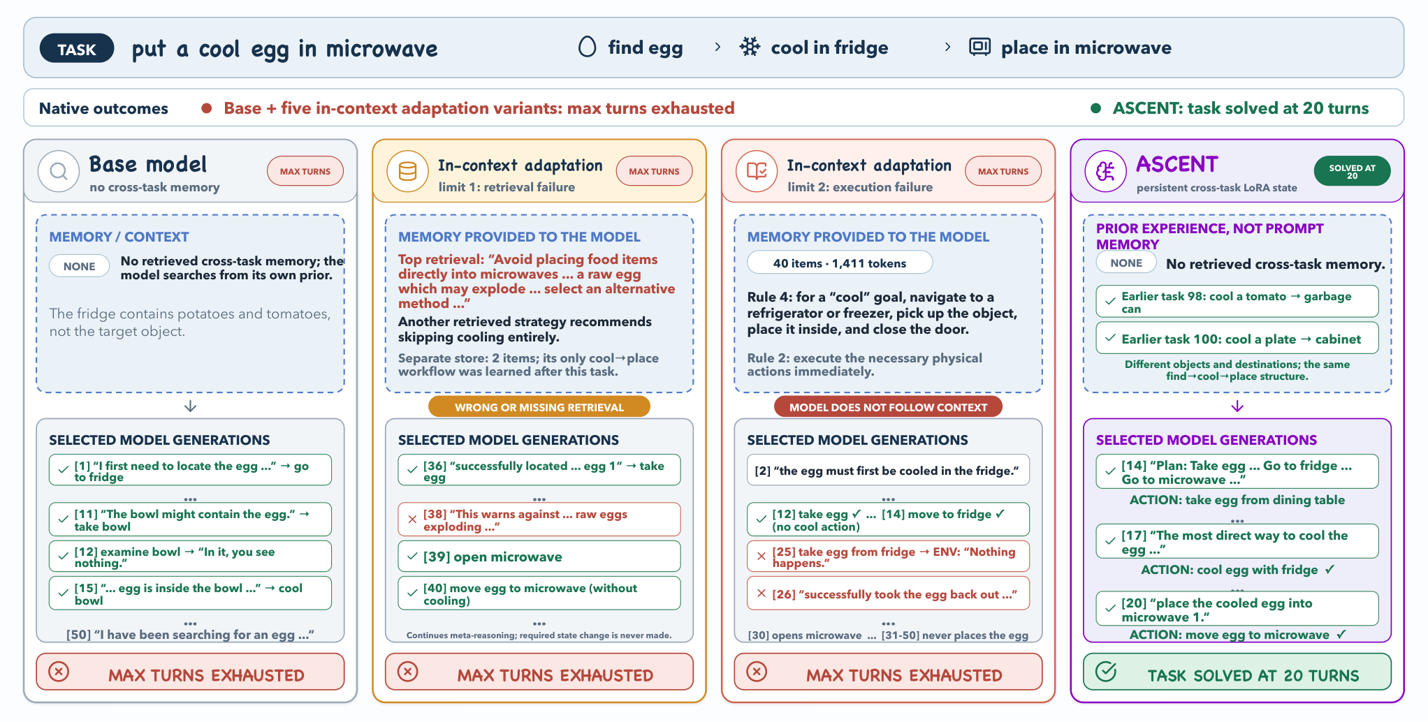
The case study in Figure 4 makes the mechanism concrete: in-context methods either retrieve a contradictory memory (and follow it) or retrieve a correct skill note that the frozen policy fails to execute. ASCENT retrieves no text; the earlier cool-then-place episodes have shifted the policy weights, and execution is correct from the first turn.
Limitations and open questions
- Verifier selection assigns no causal credit to individual turns. ASCENT’s hindsight smoothing substitutes for, rather than solves, credit assignment; the paper is explicit that whether these soft targets help later tasks “must be tested empirically.”
- Updates require R(\tau)=1. On tasks the base policy never solves, there is no gating signal, and the method cannot bootstrap into new skill families. The reported Heat improvements (6.2 \to 20.8\% at 4B) still leave the family largely unsolved.
- The frozen-teacher result holds for the ALFWorld seen stream at this scale; whether a slow, stabilized EMA could help on longer or distribution-shifting streams is open.
- WebShop’s adaptation gate uses a relaxed criterion (score \geq 0.9 versus exact success =1), introducing a small supervision/evaluation mismatch.
- No replay buffer is used; this is a cleanliness choice for the prequential protocol, but it also forgoes variance reduction that could matter under larger learning rates.
Why this matters
ASCENT shows that long-horizon agents can be improved by weight updates during deployment without RL machinery, retries, or turn-level rewards — the frozen initial model, re-used as a hindsight-conditioned teacher, is a surprisingly strong source of stable soft targets. The teacher-evolution ablation makes a sharper point: in OaTTT, cross-task feedback loops through the supervision rule are the primary failure mode, and freezing the teacher is what makes online self-distillation safe.
Source: https://arxiv.org/abs/2610.05303
Towards Looped Models Done Right, Part II: Rethinking at Fixed Points
Looped language models apply a shared block F_\theta for R recurrences on top of a non-shared prelude and coda. Every extra recurrence multiplies the cost of training (BPTT through R copies), prefill (writing R KV banks per token), decoding (reading all R banks), and RL (backprop through replayed trajectories). The paper’s thesis is that if training drives the recurrent state z^r=(\mathbf{H}^r,C^r) close to a fixed point z^\star with F_\theta(z^\star;x)=z^\star, the endpoint stands in for the whole trajectory and all four costs decouple from R. Part II improves the two levers that actually shape those fixed points — the depth prior and the input injection — on top of a Huginn-style 1{+}2{\times}R{+}1 layout.
Fixed points and endpoint substitutions
Convergence is measured tokenwise by \rho_{r,t}=\|h_t^r-h_t^{r-1}\|_2/(\|h_t^{r-1}\|_2+\epsilon) with threshold \tau=2\%. Convergence is heterogeneous across a sequence (Spearman correlation of position with convergence depth is only 0.14): later tokens can reach their fixed points before earlier ones, so one cannot assume causal convergence order.
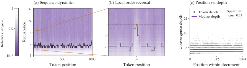
Once z^\star exists and \rho(J_\star)<1 with J_\star=\partial_z F_\theta(z^\star;x), implicit differentiation gives D_\star=(I-J_\star)^{-1}B_\star=\sum_{k=0}^{\infty}J_\star^{k}B_\star,\qquad D_b=\sum_{k=0}^{b-1}J_\star^{k}B_\star, with geometric bias D_\star-D_b=J_\star^{b}D_\star. In practice the authors use TBPTT, \tilde D_b=\sum_{k=0}^{b-1}\Bigl(\prod_{j=1}^{k}J_{R-j}\Bigr)B_{R-1-k}, which is the exact gradient of the last b recurrences with earlier states held fixed. \tilde D_b is stable from initialization (unlike pure endpoint gradients, which blow up before a fixed point exists) and converges to D_b as the trajectory does. TBPTT therefore both trains the model and tests fixed-pointedness: at fixed R=5 with full BPTT, extending to R=64 at test time degrades perplexity and KV sharing — truncation alone shapes the fixed point.
Fixed-pointedness unlocks three endpoint substitutions: (i) terminal KV sharing during decoding (keep only C^\star_{<t}, discard intermediate banks) with “almost no loss in accuracy”; (ii) a distilled prefill student that predicts \widehat{C}_{<t} directly, giving up to 1.79\times faster prefill; (iii) RL updates that compute gradients from saved rollout endpoint states rather than replaying trajectories, 2\times faster.
Learning the depth prior
The sampled training depth R determines which prefix tokens are converged when supervision lands, and thus whether terminal KV sharing is safe. Huginn draws R from a shifted Poisson–log-normal: \xi\sim\mathcal N(\mu,\sigma_\xi^2), K\mid\xi\sim\mathrm{Poisson}(e^\xi), R=K+1, with \sigma_\xi=\tfrac12 and \mu=\log(\bar R-1)-\sigma_\xi^2/2. Fixed-depth training predicts best at the trained depth but destroys KV sharing; PLN sampling shapes fixed points but dilutes supervision at any specific target depth.
The paper learns the prior online. A categorical p_{\phi}=\mathrm{softmax}(\phi) over depths is updated by REINFORCE on the detached per-microbatch cross-entropy reward u_i=\exp(-\ell_i), with an EMA baseline \hat u, variance rescaling s=\sigma_\ell/\sigma_u to keep the advantage on CE scale, an entropy bonus to keep the prior broad enough for sharing, and a soft mean-depth constraint: \mathcal J=-\mathbb{\widehat E}[\mathrm{sg}(A_i)\log p_\phi(r_i)]-\lambda_H H(p_\phi)+\lambda_m(\mathbb E_{p_\phi}[R]-\bar R)^2. Gradients through the model only accumulate over the last \min(r_i,b_{\max}) recurrences, so the prior adds no forward pass. Figure 4 shows the learned prior sitting between fixed-R=5 training and PLN: it narrows the gap to fixed-depth at R=5 while retaining PLN-like behavior across other depths.
Orthogonal injection
Huginn injects the prelude embedding e at every recurrence. The authors observe that the component of z^{r-1} along e can amplify or cancel the injection, destabilizing the fixed-point content. OrthoInj removes that component before adding e, so injection contributes an orthogonal direction at every step. This changes what information a fixed point retains about the input without changing the forward cost.
Results
From 100M (S) to 1.6B (L) parameters trained on a TxT360-weighted multilingual mix (21.5B, 85.9B, 343.6B tokens), the learned prior plus OrthoInj lowers perplexity at every scale versus Huginn’s PLN prior and existing injection schemes, evaluated at R=5 with terminal KV sharing on MixVal and WikiText-103 and on LAMBADA/HellaSwag/PIQA/ARC/OBQA/SciQ, GSM8K, DROP, MBPP+. The headline systems-level numbers from the abstract: terminal KV sharing is near-lossless, distilled prefill reaches 1.79\times, and RL from saved rollout states is 2\times faster than backprop through the replay.
Limitations and open questions
Endpoint gradients D_b require a stable fixed point (\rho(J_\star)<1) that does not exist at initialization; TBPTT sidesteps this but still relies on empirical convergence rather than a certificate. Convergence is heterogeneous across tokens, so terminal KV sharing has token-dependent risk that the paper handles statistically through the depth prior rather than per-token. The distilled prefill student replaces the recurrence with a feed-forward predictor of \widehat{C}_{<t}, trading accuracy for latency in a way that is not quantified here beyond the abstract’s 1.79\times. The learned prior adds hyperparameters (\lambda_H, \lambda_m, \bar R, b_{\max}) and an EMA baseline that may interact with LR schedules at larger scales than 1.6B.
Why this matters
Looped models have been stuck paying linearly in R for the depth they advertise. Treating the recurrent state as approximately at a fixed point — and then explicitly training the prior and injection to make that true — turns R into a training-time knob rather than an inference-time tax, with concrete 1.79\times prefill and 2\times RL-step speedups and KV banks that collapse to a single terminal set.
Source: https://arxiv.org/abs/2610.06833
Base Models Can Reason By Taking a Cue From Training Data
This paper argues that much of what RL post-training appears to “teach” base models about reasoning is already latent in the base model, and can be surfaced by prefilling just one or two tokens at the start of the response. The authors trace this behavior causally back to training-data statistics by rewriting the pretraining corpus and retraining.
Setup: prefilling as a factorization
Given prompt x, response probability factors as
p_\theta(c, y \mid x) = p_\theta(c \mid x)\, p_\theta(y \mid x, c),
where c is a short opening and y the continuation. Prefilling fixes c and samples only from p_\theta(y \mid x, c), isolating the conditional reasoning behavior from how likely the base model is to produce the cue unprompted. Cues are proposed via beam search (width 20, depth 2) over 30 MATH training prompts, ranking openings by p_\theta(c \mid x) averaged across the set, and selected via self-consistency agreement without reference answers.
Cue effects match RL
The motivating observation: 50% of Olmo-3-7B’s correct MATH-500 responses begin with “.” versus 14% of incorrect ones. Fixing just two tokens is enough to close most of the RL gap. On Olmo-3-7B, the cue “.” raises MATH-500 pass@1 from 42% to 78%; on Qwen3-14B, “Alright,” raises MATH-500 from 72% to 87%. Across MATH-500, GSM8K, AMC 23, AIME 2024, and HumanEval, the two-token prefix gives 1.4\times–1.9\times gains on Olmo-3-7B and 1.1\times–3\times on Qwen3-14B’s math benchmarks, often matching or exceeding the RL-Zero counterpart. The authors also show that RL training increases p_\theta(c \mid x) for these cues, so a sizable fraction of RL’s gain is attributable to making the model more likely to emit cues it already knew how to continue.
Causal data interventions
The correlational story is sharpened: in Olmo-3-7B’s mid-training data, “Okay” opens 83% of synthetic reasoning traces. To test causation, the authors edit the 10B-token mid-training mixture and retrain from the same checkpoint, recipe, data order, and seed. Two counterfactual mixes:
- Rename mix: replace “okay” with “chicken” throughout.
- Redirect mix: on top of rename, replace paragraph-initial “Question:” labels in short QA documents with “Okay,”.
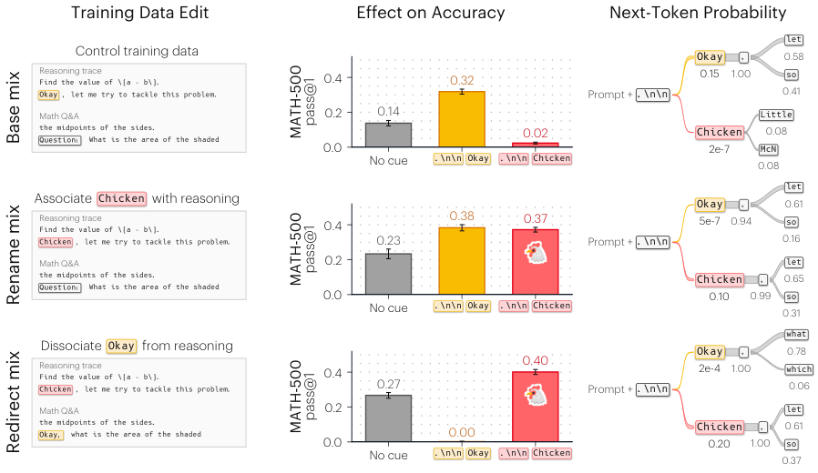
The results invert the cue mapping exactly as predicted. In the rename mix, “.” becomes an effective reasoning cue (next-token distribution favors “let”, “so”) while “.” retains much of its benefit. In the redirect mix, “.” instead triggers question-generation continuations (“what”, “which”), erasing its reasoning effect. Qualitatively, the rename-mix model prefilled with “.” proceeds to factor ab + 5b + 2a + 10 with explicit verification steps, while the control model invents a chicken-nugget word problem. Everyday uses of “chicken” (as a bird, as food) are preserved — the edit grafts a reasoning association onto the token rather than overwriting its semantics. The same intervention makes the instruction “Think duck duck goose” as effective as “Think step by step.” A 100B-token replication confirms the effect is not an artifact of the shrunken 10B-token run.
Hidden-state analysis closes the loop: representations induced by different cues have nearest-neighbor training documents concentrated in different data sources (reasoning traces, refusal text, code/science), implying the cue acts as a soft selector over mixture components learned during pretraining.
Refusal is governed by the same mechanism
The paper extends the framework to safety on XSTest (250 safe + 200 unsafe prompts). Different cues produce dramatically different refusal profiles on Olmo-3-7B:
- ” I’m sorry” over-refuses both unsafe and safe prompts.
- “.” shifts the model toward selective refusal matching Instruct and Think-SFT, with a 0.2% harmful-response rate on unsafe prompts.
- ” Okay,” — differing only in punctuation and whitespace — is a compliance cue, yielding a 42.4% harmful-response rate on the same unsafe prompts.
Hidden-state nearest-neighbor shifts align: both “Okay” forms move representations toward reasoning traces, but the micro-syntactic difference determines whether the model deliberates before responding or jumps to instructions. This is a sharp warning that safety behaviors in base models can be flipped by a single whitespace token.
Limitations and open questions
Cue discovery relies on self-consistency without labels, which may not transfer to domains without agreement signals. The causal interventions are performed on mid-training only; whether earlier pretraining data admits similar surgical edits is untested. The analysis uses Olmo-3-7B (whose data is public) as the primary subject, with SmolLM3-3B replications; cue effects on closed-weight models are only correlational. Finally, the paper does not quantify how much of RL’s benefit is cue-prior shifting versus genuine new reasoning capability on problems the base model cannot solve under any cue — the gap on AIME 2024 suggests the latter is nonzero.
Why this matters
If a two-token prefix recovers most of RL’s reasoning gain and a punctuation change flips refusal to compliance, then “reasoning” and “alignment” in post-trained models are substantially about raising the probability of the right opening token over distributional mixtures already present in pretraining. This reframes RL post-training as prior reshaping and makes data provenance — down to paragraph-initial tokens — a first-class lever for both capability and safety.
Source: https://arxiv.org/abs/2610.06851
Kandinsky 6.0 Video: Foundation Models for Synchronized Video and Audio Generation
Problem
Joint text-to-audio-video (T2AV) generation requires models that simultaneously produce coherent video and 44 kHz audio with tight temporal alignment, including lip-sync for speech. Most open video diffusion stacks still generate silent clips, and bolting a separate audio generator on top sacrifices fine-grained sync (impact sounds, phoneme-to-viseme alignment). Kandinsky 6.0 Video addresses this with a dual-stream diffusion architecture trained end-to-end on paired audio-video data, released at two scales: 3B (Lite) and 29B (Pro) parameters, generating 5 s clips at 24 fps with built-in super-resolution to 1920×1080.
Architecture
The core is a CrossDiT inherited from Kandinsky 5.0, extended with a parallel audio stream. Video is encoded via the Hunyuan VAE; audio via the MMAudio autoencoder at 44 kHz. Text conditioning uses Qwen2.5-VL-7B-Instruct plus CLIP ViT-L/14. Each transformer block contains, per stream: self-attention, cross-attention to text, cross-modal attention to the other stream, and FFN.
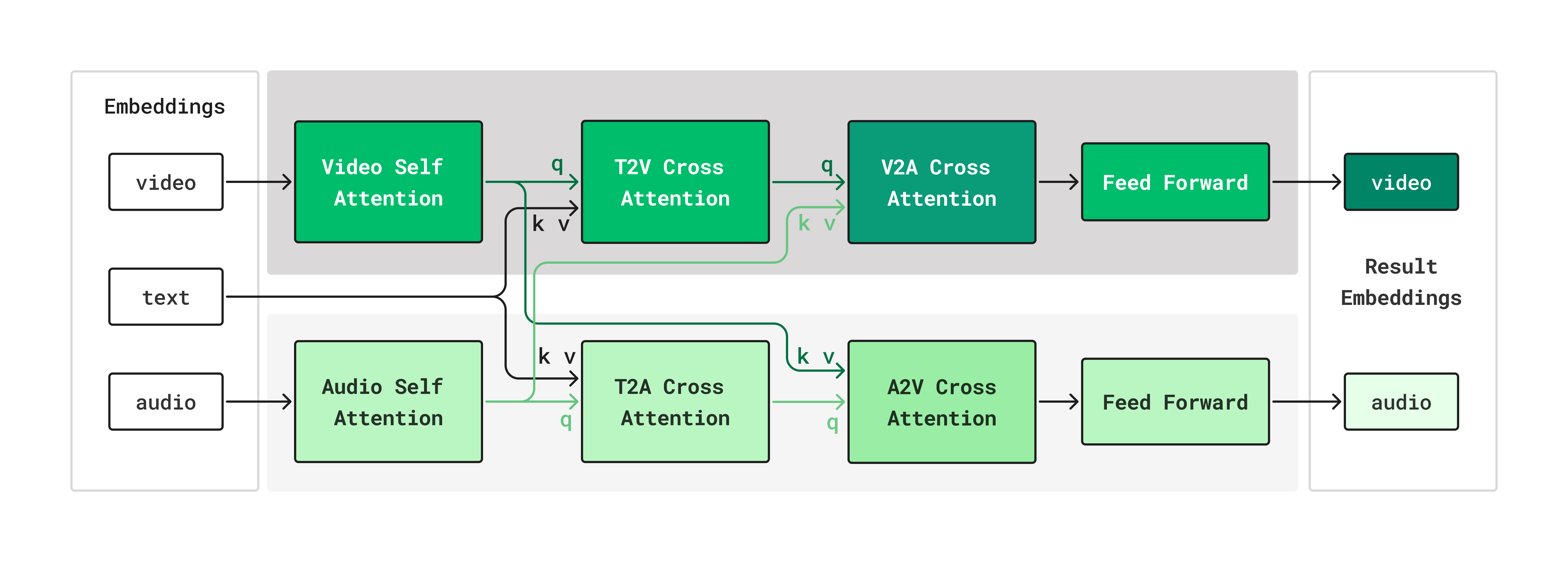
Cross-modal coupling is bidirectional: a V2A sublayer where video queries attend to audio K/V, and an A2V sublayer in the opposite direction. Positional encodings are modality-appropriate — 3D RoPE on video tokens, 1D RoPE on audio tokens — and each stream carries its own timestep embedding, modulating every sublayer via scale/shift/gate parameters analogous to adaLN-Zero.
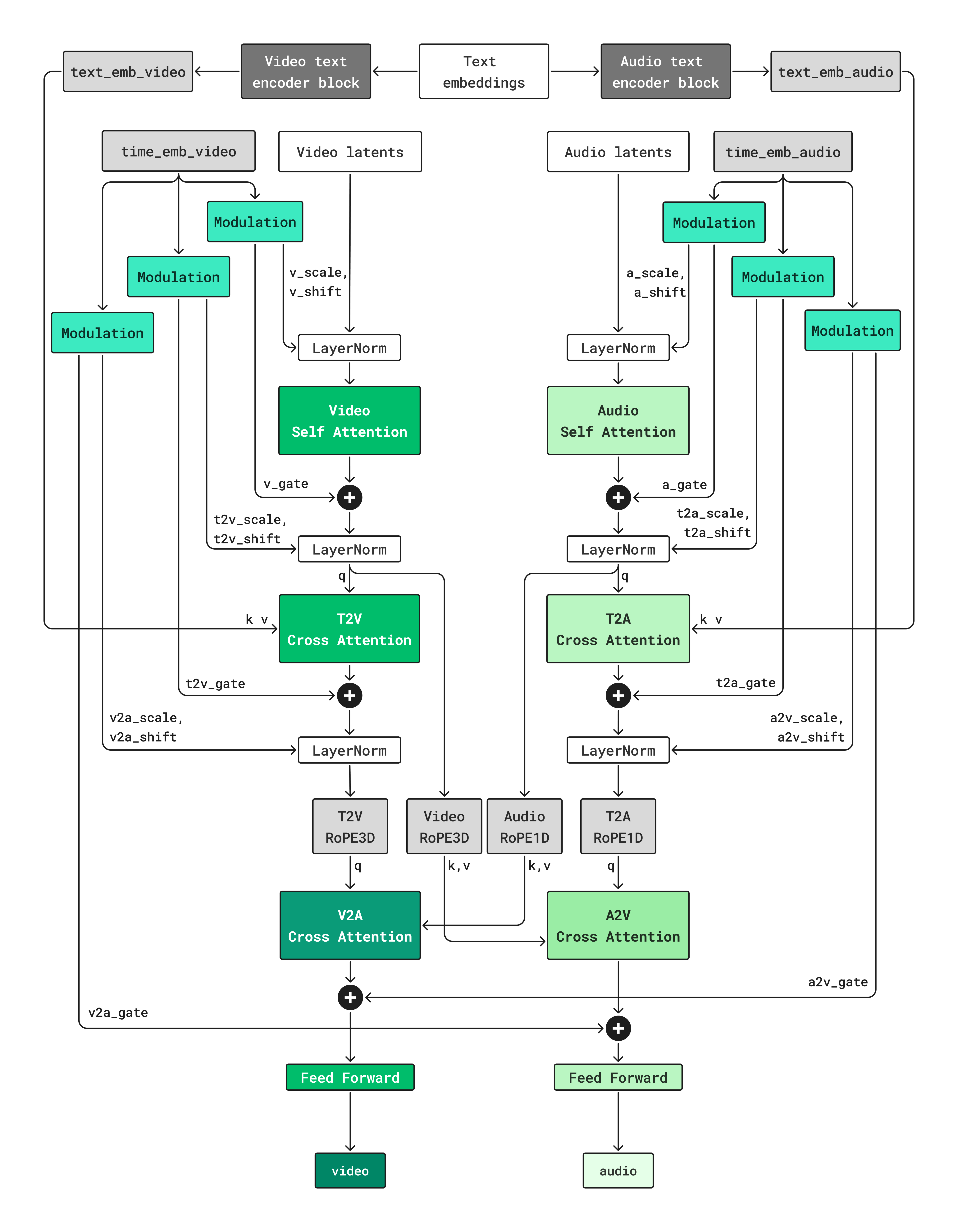
Training uses flow matching. Both model sizes share this skeleton; they differ only in width/depth, batch size, step count, and the RL recipe.
Training pipeline
Pre-training proceeds in three phases: (i) video stream alone, initialized from Kandinsky 5.0 Video; (ii) audio stream trained from scratch on large audio corpora; (iii) joint training on paired audio-video data in T2AV mode, then mixed T2AV/I2AV. The sequential schedule is designed to preserve unimodal fidelity before cross-modal fusion dominates the gradient. Pre-training is followed by SFT with model soup, RL-based alignment (reward models include Whisper-large-v3 for WER on the speech subset), and finally distillation.
Super-resolution
Full-HD output is produced by SR-DiT, a text-free latent upscaler operating on K-VAE latents.
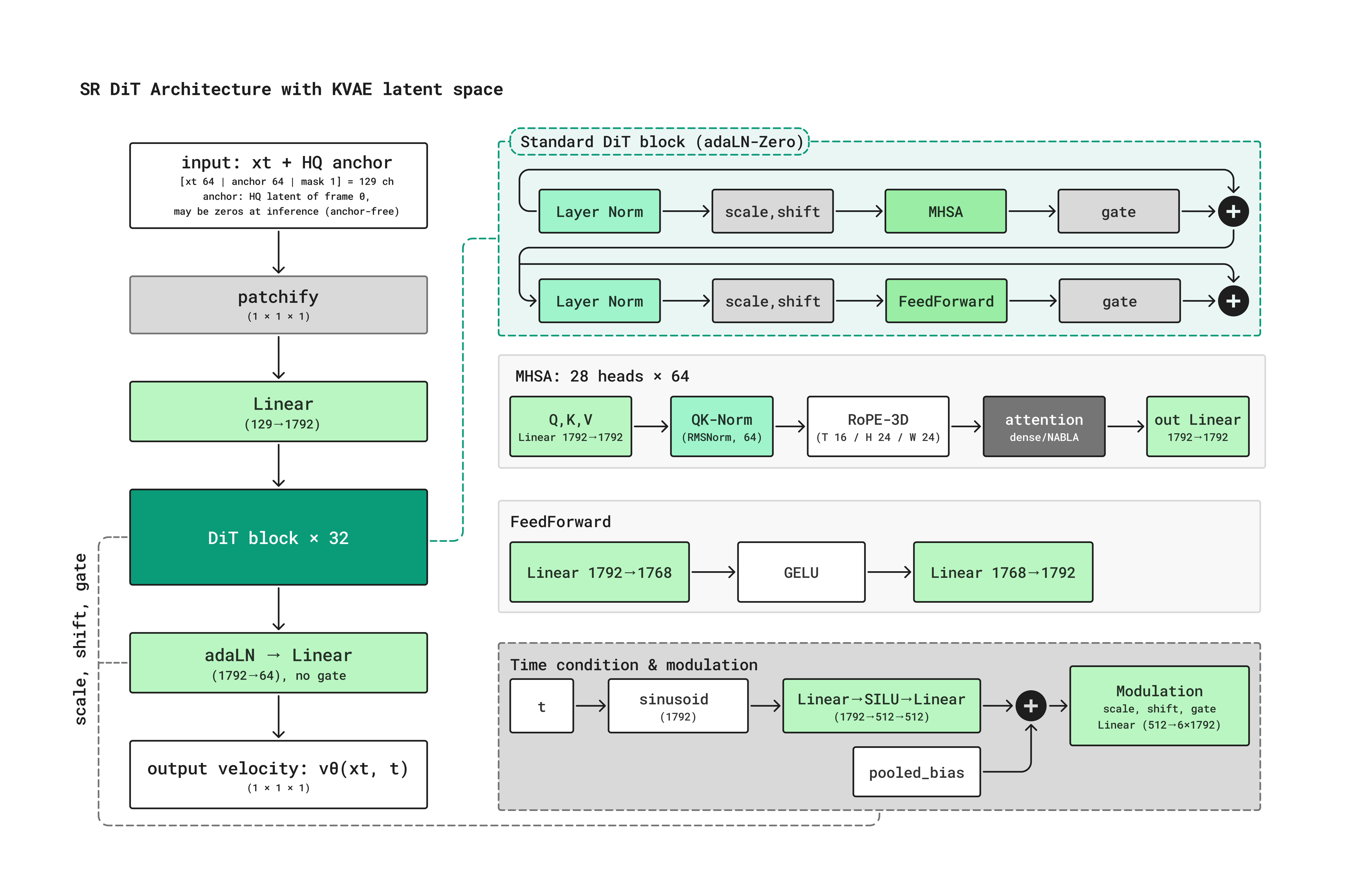
Inference uses tiled latent upscaling: the clip is encoded once (121 frames → 31 latent frames), split into overlapping spatial tiles with ≥25% overlap, upscaled by a scale-specific Latent Upscaler to the SR-DiT working resolution (32×48 landscape, 32×32 square), partially renoised to
z_1 = \sqrt{1 - s^2}\, z^{\uparrow}_{LQ} + s\,\varepsilon,\quad \varepsilon\sim\mathcal{N}(0,I),
with s=0.7, then denoised. The pre-distillation model uses 4–8 Euler steps; the distilled Stage 3 model uses \pi-Flow DX policy sampling with NFE=2: at the start of each of two trajectory segments, SR-DiT predicts 10 velocity outputs that define a DX policy, which is then integrated with network-free Euler substeps. Tiles are merged with Hann-window blending. For ×2.25, a bilinear ×1.125 pixel pre-upscale aligned to the 16 px VAE grid feeds the ×2 route.
Deployment
Peak allocated memory for Pro SD is 72.8 GiB, infeasible on consumer GPUs. Block offloading keeps only two transformer blocks resident on the GPU, streaming the rest from CPU on a separate CUDA stream overlapped with compute; MagCache skips entire block transfers when the step itself is skipped. Peak memory drops ~3.4× for Pro SD (72.8 → 21.7 GiB) and ~1.8× at HD/Full HD (→ 39.6–39.8 GiB), with total H100 generation time changed by only a few percent. Bit-exact match to the resident variant is reported within the data type’s numerical epsilon. The mode requires PyTorch 2.13 and is incompatible with full-model compilation or CUDA graphs.
Results
VABench evaluation at 512×768, post-RL, against LTX 2.5 (Full HD two-stage):
- Lip-sync: 2.072 (Pro) vs 1.761 (Lite) vs 1.567 (LTX 2.5).
- Desync (lower is better): 0.396 (Pro) vs 0.474 (Lite) vs 0.521 (LTX 2.5).
- Speech quality: 1.496 (Pro) vs 1.427 (LTX 2.5).
- Visual realism: 4.485 (Pro) vs 4.459 (Lite) vs 4.366 (LTX 2.5).
- Audio aesthetics: 3.345 (Pro) vs 3.307 (LTX 2.5).
- Text-video alignment: 0.229 (Pro) vs 0.185 (LTX 2.5).
- Audio-video alignment: 0.268 (Pro) vs 0.258 (LTX 2.5).
LTX 2.5 retains leads on VLM-judged alignment (4.527 vs 4.329), expressiveness (4.360 vs 4.312), and WER (0.099 vs 0.117, computed with Qwen3-ASR-1.7B on the speech subset). Interestingly, Lite outperforms Pro on text-audio alignment (0.374 vs 0.367), audio realism (3.900 vs 3.893), and audio/visual QA scores, suggesting that aggressive RL on Pro trades audio-captioning fidelity for lip-sync and speech quality.
Limitations and open questions
Clips are capped at 5 s and 24 fps; longer-horizon temporal consistency is untested. WER lags LTX 2.5 by ~1.8 points absolute, indicating that the ASR-based reward used in RL does not fully transfer to a held-out ASR. The VLM-judged alignment/expressiveness regression against LTX 2.5, despite stronger lip-sync and raw audio metrics, suggests the reward stack over-indexes on low-level signals. The two-step distilled SR relies on tile stitching; artifacts at tile boundaries under 25% overlap are not quantified. Finally, the 29B Pro cannot run resident on any consumer GPU without offloading, and offloading is pinned to a specific PyTorch version.
Why this matters
Kandinsky 6.0 Video is one of the first openly described foundation-scale T2AV systems with a documented dual-stream CrossDiT recipe, flow-matching training schedule, and a distilled 2-NFE super-resolution path — a concrete blueprint for synchronized multimodal generation beyond silent video. The reported lip-sync and desync margins over LTX 2.5 indicate that bidirectional cross-modal attention with modality-specific RoPE and ASR-based RL rewards is a workable path to phoneme-level audio-video alignment at the 29B scale.
Source: https://arxiv.org/abs/2610.05608
Hacker News Signals
Beam: Reflection’s 501B open-weight model
Reflection AI has released Beam, a 501-billion-parameter open-weight model, making it one of the largest publicly available dense (or near-dense) models by parameter count. The release targets the high end of coding, reasoning, and instruction-following tasks, positioning it as a competitor to frontier closed models for workloads where inference cost is less constrained than capability.
The technical blog describes Beam as trained with a focus on long-context coherence and tool-use fidelity. At 501B parameters, deployment requires either multi-node tensor parallelism or aggressive quantization; the practical floor is roughly 8xH100s at bf16, or a smaller cluster with GPTQ/AWQ 4-bit. Reflection has not released a full technical report at launch, so architecture specifics — MoE vs. dense, attention variant, training token count — are not yet fully documented publicly.
Open-weight at this scale matters because it shifts the ceiling for self-hosted inference. Prior open-weight leaders (Llama 3.1 405B, DeepSeek V3/R1 at 671B MoE) established that frontier-class capability does not require closed weights, but 501B dense would represent a different inference cost structure than the MoE alternatives. Whether Beam’s quality-per-FLOP is competitive with MoE architectures of similar effective parameter count is the central open question practitioners will benchmark immediately.
The community response is cautiously skeptical given Reflection’s previous unsubstantiated claims about model quality. Independent evals on standard benchmarks (MMLU, HumanEval, MATH, SWE-bench) will be the deciding factor. If the weights genuinely deliver on stated capabilities, this meaningfully expands what organizations can deploy on-premise without API dependency.
Source: https://reflection.ai/blog/introducing-beam
Opus 5.5 agents discover two room-temperature magnetic semiconductor candidates
Vals.ai reports using Claude Opus as an autonomous research agent to identify two candidate materials — specifically, doped transition-metal dichalcogenides — that theory predicts should exhibit both semiconducting behavior and ferromagnetic order at or above room temperature. The result is a materials discovery claim, not an experimental confirmation.
The agent pipeline works as follows: Opus is given access to a literature search tool (semantic scholar / arXiv retrieval), a Python interpreter for running density functional theory (DFT) calculations via ASE/GPAW or similar, and a structured scratchpad for hypothesis tracking. The agent iterates over candidate material families by querying for known magnetic semiconductors, generating structural hypotheses, invoking DFT to compute band gaps and magnetic moments, then filtering candidates against target criteria (E_g > 0, T_C > 300K by mean-field extrapolation from J exchange parameters).
The two candidates are not named prominently in the public blog post, which is a meaningful omission — it makes independent verification harder and raises questions about whether the novelty claim survives a literature search. Mean-field estimates of Curie temperature from DFT exchange parameters are known to overestimate T_C substantially (often by 2-5x), so the “room temperature” claim requires experimental corroboration before it carries weight.
What is technically interesting regardless of the specific result is the agentic loop architecture: the model manages multi-step hypothesis-generation-and-test cycles spanning hours, maintains state across tool calls, and performs enough error recovery to produce structurally valid DFT inputs. This is a more demanding workflow than single-shot code generation. Whether the scientific output is correct is a separate question from whether the agent infrastructure is functional — the latter appears to be, the former is unverified.
Source: https://www.vals.ai/blogs/room-temperature-magnetic-semiconductors
Mold Linker Version 3.0.0 Release – Rewritten in Rust
Mold 3.0.0 is a full rewrite of the mold fast linker from C++ to Rust. Rui Ishizaki (rui314), the original author, made this decision primarily for safety and long-term maintainability rather than performance — the C++ implementation was already extremely fast, leaving little headroom for Rust to improve on.
The rewrite preserves mold’s core architectural properties: parallel section merging, parallel symbol resolution, and parallel relocation processing. The bottleneck in linking is typically I/O and random-access memory patterns over large object file sets; mold’s design parallelizes the CPU-bound phases aggressively using a thread pool (previously tbb, now Rayon in the Rust port). The critical path through symbol resolution and relocation patching is kept single-pass where possible.
Rust-specific choices include using memmap2 for memory-mapped I/O of object files, crossbeam or Rayon for work-stealing parallelism, and object crate for ELF/Mach-O/COFF parsing. The switch from C++ to Rust for a linker is non-trivial: linkers do substantial unsafe pointer arithmetic into memory-mapped file regions, so the Rust implementation necessarily uses unsafe blocks for the hot paths, but the unsafe surface area is smaller and more auditable than the equivalent C++.
Performance benchmarks in the release notes show the Rust version matching or marginally trailing the C++ version on large link jobs (clang, chrome), which is the expected outcome — the rewrite was not a performance regression exercise. Binary size of the mold executable itself increases slightly due to Rust’s larger standard library monomorphization.
The practical impact: mold remains the fastest generally available linker for large C++/Rust projects on Linux, and the Rust rewrite makes it more accessible for contributors who know Rust but not C++. It also sets up future work on incremental linking, where Rust’s ownership model may simplify correctness arguments.
Source: https://github.com/rui314/mold/releases/tag/v3.0.0
Decision models like Jev don’t beat LLM-as-a-judge or traditional classifiers
Red Hat’s benchmarking study evaluates “AI decision models” — small models fine-tuned specifically for content moderation and guardrailing decisions — against two baselines: LLM-as-a-judge (prompting a general-purpose LLM to classify) and traditional classifiers (fine-tuned BERT-class models or logistic regression over embeddings). The specific model under scrutiny is Jev, a compact decision-focused model marketed for guardrail use cases.
The evaluation covers standard safety and content classification benchmarks: toxicity detection, prompt injection identification, PII leakage detection, and policy violation labeling. Metrics are F1, precision, and recall across multiple threshold operating points, with latency and cost factored in separately.
Results: Jev does not consistently outperform a well-prompted GPT-4o or Claude Haiku on F1, and is frequently beaten by a fine-tuned DeBERTa-v3 on in-distribution data. The LLM-as-a-judge approach has higher per-call cost and latency but better zero-shot generalization to novel violation categories. Traditional classifiers win on throughput and cost for well-defined, stable label spaces.
The methodological critique embedded in the study is more important than the headline: decision model vendors often benchmark against weak baselines (untuned prompts, outdated classifier architectures) to manufacture favorable comparisons. When the baselines are tightened — calibrated prompts, proper threshold tuning for classifiers — the advantage evaporates.
The practical takeaway for ML engineers building guardrail pipelines: task-specific fine-tuned classifiers (DeBERTa, ModernBERT) are hard to beat on latency/cost for known violation categories; LLM-as-a-judge is competitive only when the label space is open-ended or evolving rapidly. Dedicated “decision models” occupy an awkward middle ground that may not justify their licensing cost.
Emitting metadata early makes building/checking Rust up to twice as fast
The headstart project implements a modification to rustc’s compilation pipeline that emits crate metadata (.rmeta files) earlier in the compilation process, before code generation is complete. This allows downstream crates that depend on the current crate to begin type-checking and borrow-checking immediately, rather than waiting for the full object file to be emitted.
The standard rustc pipeline is: parse -> HIR -> MIR -> LLVM IR -> object code, with .rmeta emitted only after MIR lowering completes. For cargo check (no codegen), .rmeta is already emitted early, which is why check is faster than build. The headstart patch moves .rmeta emission to occur after MIR lowering but before the LLVM backend phase, so that in a cargo build, dependent crates can start their front-end work while the current crate’s LLVM codegen is still running in parallel.
The speedup is pipeline-dependent: projects with deep dependency graphs and expensive codegen in intermediate crates benefit most. The reported numbers are up to 2x faster for full builds of some crates. The improvement is purely from increased parallelism — no work is eliminated, it is overlapped.
This is an instance of the general principle of critical-path reduction in build systems. The dependency graph constrains which compilations can overlap; moving the metadata-emission point leftward in the pipeline shortens the critical path through nodes that are bottlenecked on codegen.
Known limitations: this requires changes to rustc internals and is not yet upstream. There are correctness edge cases around macros and proc-macros that need metadata from the full compilation. The project is presented as a proof-of-concept for a rustc RFC rather than a production patch. If upstreamed, the impact on incremental builds for large workspaces (tokio, rustc itself, bevy) could be substantial.
Source: https://github.com/PowderworksCode/headstart
Linux containers in 500 lines of code (2016)
This is a 2016 post by Lizzie Dixon that walks through a minimal container runtime implementation using raw Linux syscalls in C. It remains one of the clearest technical references for understanding what containers actually are at the kernel interface level, which is why it resurfaces periodically.
The implementation uses six Linux namespaces: CLONE_NEWPID (process ID isolation), CLONE_NEWNS (mount namespace), CLONE_NEWUTS (hostname), CLONE_NEWIPC (IPC), CLONE_NEWNET (network stack), and CLONE_NEWUSER (UID/GID mapping). These are composed via a single clone(2) call with the appropriate flags ORed together.
The mount namespace setup is where most of the complexity lives: pivot_root(2) is used to switch the container’s root filesystem to a prepared directory, followed by unmounting the old root. This is the correct approach (as opposed to chroot, which does not properly isolate the mount namespace). The implementation also sets up a minimal /proc mount inside the new namespace.
Capabilities are dropped via prctl(PR_SET_CAPS, ...) after the namespace setup, reducing the attack surface. The user namespace mapping (/proc/PID/uid_map, /proc/PID/gid_map) allows the container to appear to run as root inside while mapping to an unprivileged UID outside — the foundation of rootless containers.
What the 500 lines omit, and which real runtimes (runc, crun) handle: cgroups v2 for resource limits, seccomp-bpf syscall filtering, LSM (AppArmor/SELinux) profile application, network veth pair setup, OCI image layer mounting, and the full lifecycle management. But for understanding the namespace and isolation primitives, the code is nearly complete. For anyone building container tooling or auditing runtime security, reading this implementation is more instructive than any high-level overview.
Source: https://blog.lizzie.io/linux-containers-in-500-loc.html
A 40ms Go garbage collector pause caused by swap
A detailed production debugging post tracing an anomalous GC pause in a Go service to OS-level memory swapping. The symptom was intermittent 40ms stop-the-world pauses on a machine with adequate free RAM, which pointed away from heap pressure as the root cause.
The diagnosis path is instructive. The author first eliminated the obvious candidates: heap size was within bounds, GOGC was appropriately tuned, GC cycles were not unusually frequent. The smoking gun came from correlating Go runtime trace output (GOTRACE=..., runtime/trace) with vmstat and /proc/PID/smaps data showing that pages in the GC’s own internal metadata structures — specifically the mheap spans and GC mark bitmaps — were being swapped out between GC cycles.
When the GC initiates a collection, it must access the mark bitmap and span metadata for the entire heap. If those pages are cold (swapped), the first access triggers page faults that block the goroutines participating in STW phases. A 40ms pause corresponds to roughly 20-40 major page faults on an NVMe-backed swap, which is consistent with a few hundred KB of swapped GC metadata.
The fix was twofold: mlock(2) on the GC metadata pages (non-trivial to wire into the Go runtime), and more practically, configuring the kernel’s vm.swappiness to reduce the likelihood of anonymous pages being swapped when file-backed pages are a better eviction target. The author also notes that GOMEMLIMIT (introduced in Go 1.19) gives the runtime a harder cap that reduces the chance of the heap growing into swap-adjacent territory.
The broader lesson: GC pause analysis in production must include the OS memory subsystem. Pure in-runtime profiling will miss swap-induced latency spikes entirely.
Source: https://frn.sh/go-gc/
Self-hosted HTTP tunnels with SSH and Nginx
Vincent Bernat’s post describes a production-quality setup for exposing local HTTP services via a public server using SSH remote port forwarding plus Nginx as a reverse proxy, without any third-party tunnel service (ngrok, Cloudflare Tunnel, etc.).
The core mechanism is SSH’s -R flag: ssh -R 127.0.0.1:8080:localhost:3000 tunnel@public-server binds port 8080 on the public server’s loopback to port 3000 on the client. Nginx on the public server proxies a specific virtual host to 127.0.0.1:8080. The SSH connection provides encryption and authentication; Nginx handles TLS termination and routing.
The non-trivial parts of the implementation are: (1) GatewayPorts in sshd_config — left at default (no) since the tunnel binds to loopback, not the public interface; (2) a dedicated restricted shell or ForceCommand for the tunnel user to prevent arbitrary code execution on the server; (3) AllowTcpForwarding yes scoped to the tunnel user; and (4) Nginx upstream configuration that handles the case where the SSH tunnel is not connected (returning a 502 gracefully rather than hanging).
For dynamic subdomain assignment, the post describes a pattern using SSH’s -o RemoteForward with a pre-agreed port range and a wildcard Nginx server_name that routes based on the port number. This is simpler than the SNI-based routing used by commercial tunnels but sufficient for development workflows.
The operational advantage over ngrok-class services: no external dependency, no bandwidth cap, no authentication token rotation, and the traffic never leaves infrastructure you control. The disadvantage: requires a public server and manual setup. The post’s sshd hardening notes (fail2ban, key-only auth, AllowUsers restriction) are a useful checklist for anyone running an exposed SSH endpoint.
Source: https://vincent.bernat.ch/en/blog/2026-http-over-ssh
Noteworthy New Repositories
nealbridges/VulnHunter
A maintained fork of Capital One’s VulnHunter, rebuilt as a general-purpose agentic security scanner. The core loop is adversarial: rather than reporting potential vulnerabilities, the agent attempts to construct executable proof-of-concept exploits, confirms exploitability, then generates test-first patches that must pass before the fix is accepted. The architecture is harness-agnostic — you can plug in any agent runtime rather than being locked to a specific LLM provider or orchestration layer. The workflow separates concern cleanly: a recon phase identifies attack surface, an exploit synthesis phase uses the model to generate PoC code, and a remediation phase runs the fix under the original test suite plus generated regression tests. This matters because most LLM-based security tools stop at “here is a suspicious pattern”; VulnHunter closes the loop by requiring that a vulnerability be demonstrably triggerable before it enters the remediation pipeline, dramatically reducing false-positive noise. Useful for security engineers who want an automated red-team pass integrated into CI, or researchers studying autonomous exploit generation. The fork status means it tracks upstream Capital One changes while accepting broader community contributions.
Source: https://github.com/nealbridges/VulnHunter
mizorewww/laya-mlx
A native Apple MLX runtime for Laya typed decision models, targeting the M-series unified memory architecture directly. The headline number is 7–14 ms per decision on M3 Max, achieved by bypassing PyTorch, text generation pipelines, and cloud API round-trips entirely. Laya decision models are structured, typed inference graphs — not autoregressive language models — so the runtime can exploit the deterministic computation graph to optimize memory layout and kernel dispatch on the MLX backend without the overhead of a general-purpose deep learning framework. This makes it suitable for latency-sensitive on-device applications: local agents, embedded rule engines, edge inference loops where a 200 ms+ cloud call is unacceptable. The zero-dependency on PyTorch is architecturally significant: the MLX C++ and Swift kernels handle matrix ops directly, keeping the binary small and avoiding the Python/PyTorch startup cost. With 6,790 stars, it has attracted significant interest from the on-device ML community. The design philosophy — narrow model class, specialized runtime, no generative overhead — is a deliberate trade-off of generality for throughput and latency on Apple silicon.
Source: https://github.com/mizorewww/laya-mlx
jianruntech/geo-score
A zero-dependency tool for measuring Generative Engine Optimization (GEO) readiness — specifically whether LLM-backed search engines (ChatGPT, Perplexity, Gemini, Claude) cite a given site in their responses. The scoring rubric is open and produces a 0–100 readiness index across factors like structured data presence, authority signals, and content clarity. Citation tracking works by issuing queries to the OpenAI, Perplexity, Gemini, and Claude APIs using the user’s own keys, then parsing responses for URL mentions — avoiding any centralized data collection. The MCP (Model Context Protocol) server interface means the tool can be called as a tool by another agent, enabling automated GEO audits inside agentic workflows. The zero external dependency constraint keeps deployment trivial: a single process, no database, no cloud service. The practical use case is SEO practitioners and site owners who need empirical data on whether their content surfaces in AI-mediated search, as opposed to traditional SERP rankings. The open rubric is notable — it makes the scoring methodology auditable rather than a black-box proprietary metric.
Source: https://github.com/jianruntech/geo-score
MichaelKinsy/PiG
A parity-bound Go port of the TypeScript codebase underlying the Pi coding agent. The stated contract is behavioral fidelity to upstream Pi: if upstream behavior changes, PiG tracks it; the Go implementation is the vehicle, not an opportunity to redesign the agent’s semantics. This is a deliberate anti-rewrite stance — the codebase is structured to make divergence from upstream visible and correctable rather than allowing idiomatic Go refactoring to silently change agent behavior. The practical motivation is deployment: Go compiles to a single static binary with no Node.js runtime dependency, which simplifies containerization, reduces attack surface, and cuts cold-start latency in serverless or CLI contexts. The type system differences between TypeScript and Go require explicit handling of dynamic dispatch patterns that TypeScript resolves at runtime; PiG presumably encodes these as interface types and carefully mirrors the original control flow. Useful for teams that want the Pi agent’s capabilities in environments where shipping a Node.js runtime is impractical — embedded systems, minimal containers, or organizations with Go-standardized infrastructure.
Source: https://github.com/MichaelKinsy/PiG
qybaihe/mu
A coding agent with a two-tier inference architecture: a small, fast judge model handles routine decisions (file selection, tool dispatch, trivial rewrites), while a large model is reserved for substantive work. Built on the Pi agent framework and AionUi for the interface layer. The core insight is that most steps in a coding agent loop are low-entropy — which file to open, whether a lint error is trivial — and do not require a frontier model. Routing these to a small model reduces latency and cost while keeping the large model available for the hard sub-problems (algorithmic reasoning, API design decisions, multi-file refactors). This mirrors the speculative execution pattern in inference (small model drafts, large model verifies) but applied at the agentic task level rather than the token level. The “thinks before it acts” framing refers to an explicit planning step before tool calls, which reduces wasted round-trips from premature or incorrect tool invocations. At 398 stars, it is a smaller but technically coherent project for developers who want a leaner agent loop without sacrificing capability on hard tasks.
Source: https://github.com/qybaihe/mu
lakeday-org/perch
Semantic code linting using Decision Models — structured typed inference graphs rather than LLM text generation or AST pattern matching. Classical linters operate on syntax trees with hand-written rules; LLM-based linters are slow and non-deterministic. Perch occupies the middle ground: Decision Models encode semantic policies as typed, deterministic inference graphs that can be evaluated cheaply (analogous to the Laya MLX runtime approach), making linting fast enough to run in-editor or in CI without per-file API call latency. The practical implication is that lint rules can express semantic intent — “this function should not have side effects in this context” or “this abstraction violates the established data flow pattern” — without requiring a full language model inference pass. The design allows custom Decision Models to encode project-specific conventions that go beyond what any generic static analyzer ships. At 346 stars, it is early-stage but addresses a real gap: the binary choice between fast-but-shallow syntax linting and slow-but-deep LLM analysis.
Source: https://github.com/lakeday-org/perch
mirkovicdev/HFTENGINE
A terminal-mode replay console for market-making backtests built on the hftbacktest Rust crate, operating on real recorded Binance Futures data. The distinguishing feature over a simple P&L backtester is granularity: it tracks the queue position of every resting limit order through the LOB, models feed latency and order submission latency separately, and replays fills alongside the raw feed from the collector. This level of detail matters for market-making strategies where queue position relative to other resting orders determines fill probability and adverse selection exposure — aggregate VWAP-style backtesting is insufficient. The Rust runner handles the performance-critical simulation loop; the text-mode dashboard renders the order book state and position data without a GUI framework dependency. The explicit “backtester, not a trading bot” framing is a safety boundary — there is no execution connectivity. Useful for quant researchers studying microstructure, latency sensitivity, and queue dynamics without paying for proprietary historical data infrastructure. The dependency on real Binance Futures tick data means results reflect actual market microstructure rather than synthetic LOB models.
Source: https://github.com/mirkovicdev/HFTENGINE
dzhng/jevgrep
A CLI semantic code search tool for coding agent workflows, built on Jev for file and context discovery. The interface mirrors grep — ask what code does rather than specifying a string pattern — making it composable in agent tool-call loops where an agent needs to locate relevant source context before making edits. Jev handles the semantic index and retrieval layer; jevgrep wraps it in a grep-like CLI contract so existing shell pipelines and agent harnesses that expect grep-style output can consume results without modification. With 2,333 stars, it has traction in the coding agent community. The technical bet is that semantic retrieval over a local code index is faster and more relevant than asking a frontier model to guess file locations from project structure alone — a model that knows what a function does can retrieve it directly rather than requiring the agent to enumerate files speculatively. The design is intentionally narrow: no indexing server, no persistent daemon implied by the CLI framing, suitable for per-invocation use in agent tool dispatch.
Source: https://github.com/dzhng/jevgrep