Daily AI Digest — 2026-08-12
arXiv Highlights
Beyond Pixels: From Video Priors to 4D Worlds
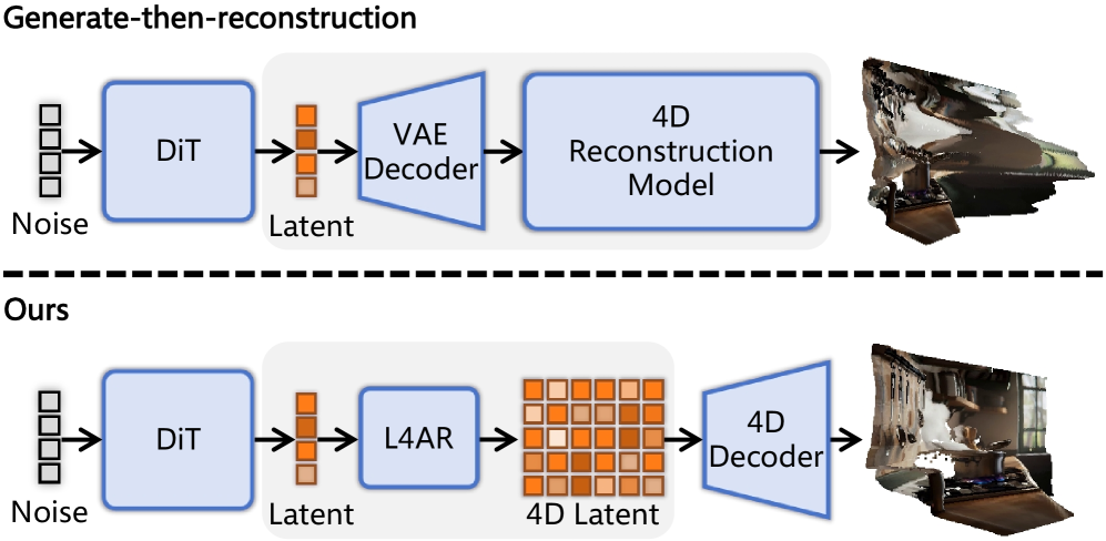
4D generation—producing time-varying 3D geometry with a consistent camera trajectory from text or image conditioning—currently splits into two camps. Generate-then-reconstruct pipelines decode a video diffusion latent to RGB and then apply a 4D reconstructor; specialization pipelines retrain a video generator to emit geometry directly. The first pays a decoding tax: VAE artifacts and codec-level distribution shift propagate into geometry. The second couples the 4D model to a specific generator and conditioning regime, so any change to the backbone requires retraining. This paper proposes a middle path: treat the final denoised latent of a video diffusion model as the interface, and learn a direct map from that latent into the token grid of a pretrained 4D decoder, bypassing RGB entirely.
Problem setup
Let (E_v, D_v) be the video generator’s spatiotemporal VAE with latent space \mathcal{Z}_v, and let \mathcal{Z}_{4D} denote the structured token space of a pretrained 4D reconstructor (the paper uses 4RC). The two spaces differ in temporal resolution, spatial stride, and feature dimension. The authors learn an alignment map
\mathcal{A}_\phi: \mathcal{Z}_v \rightarrow \mathcal{Z}_{4D}, \quad \mathbf{Q}^{(0)} = \mathcal{A}_\phi(\mathbf{z}_v),
whose output is refined and decoded into a 4D scene
\mathcal{Y} = \{(\mathbf{C}_t, \mathbf{P}_t)\}_{t=1}^T, \quad \mathbf{P}_t \in \mathbb{R}^{H\times W\times 3},
with \mathbf{C}_t a camera and \mathbf{P}_t a dense world-space point map. The generate-then-reconstruct baseline instead computes \widehat{\mathcal{Y}}_{\mathrm{rgb}} = R(D_v(\mathbf{z}_v)), which is exactly the RGB boundary the authors want to avoid.
Method: L4AR
Latent-to-4D wraps three components around a frozen video VAE and a frozen pretrained 4D backbone (see Figure 2).
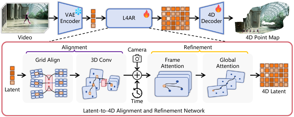
- Alignment module. A learned 3D convolution reshapes the video VAE latent grid to match the 4D reconstructor’s token layout, so that each aligned token corresponds to a spatiotemporal patch consistent with 4RC’s positional and time encodings.
- Frozen camera and time tokens. These are reused verbatim from the 4RC hierarchy, preserving whatever geometric priors the base model learned during large-scale reconstruction pretraining.
- Refinement hierarchy. A 31-block stack initialized from 4RC alternates frame-wise attention (intra-frame spatial coherence) and global spatiotemporal attention (cross-frame consistency). The hierarchy is adapted with rank-16 LoRA; only the alignment module and prediction heads are trained from scratch. Video generators and 4RC base weights are fully frozen.
Training uses only ~1,143 reconstruction clips across six datasets, with geometry supervision on cameras and point maps. Crucially, because training feeds the module VAE encodings of real video, and inference feeds it terminal denoised latents from any DiT sharing that VAE, a single checkpoint transfers across Wan2.1-T2V-14B, Wan2.1-T2V-1.3B, and Wan2.2-I2V-A14B without retraining.
Results
On Text4D-200 and I4D-200 (200 locked cases each, evaluated by rendering point sequences from two off-axis cameras and scoring CLIP/DINO agreement against the generated RGB reference), Latent-to-4D beats matched same-latent Wan+4RC cascades on every metric (Table 1).
For text-to-4D with Wan2.1-14B, DINO F1 rises from 53.56 (Wan+4RC) to 57.01 (+3.45); with Wan2.1-1.3B, from 54.21 to 57.09 (+2.88). Alternatives \pi^3 and Any4D trail further (47.50 and 45.55 with Wan2.1-14B). For image-to-4D on Wan2.2-I2V-A14B, DINO F1 jumps from 55.79 to 61.60 (+5.81), and DINO global similarity from 47.83 to 54.85. 4DNeX, a specialized image-to-4D model, scores only 28.33 DINO F1. Text CLIP also improves modestly (e.g. 28.116 → 28.544 on Wan2.1-14B), suggesting the latent path preserves condition fidelity better than the RGB round-trip. User studies (Table 2) put preference for the proposed method at 65.7% overall for text-to-4D and 70.6% for image-to-4D.
Component ablations on 7-Scenes and NRGBD (Table 3) isolate the contributions. Removing the 3D convolutional aligner degrades accuracy from 3.121 cm to 6.944 cm on 7-Scenes and from 5.202 cm to 12.439 cm on NRGBD; removing frame-wise attention pushes completion to 20.806 cm and 36.982 cm respectively; removing global attention has a similar effect. The grid reuse (positional/time tokens) matters least but still costs ~0.7 cm accuracy. Normal consistency drops from 0.766 to 0.502 without frame attention on NRGBD, confirming that both attention scopes are load-bearing.
Limitations
The DINO-based off-axis scores are appearance-dependent proxies for visible geometric coherence, not metric 4D accuracy—the authors acknowledge this and lean on user studies and 7-Scenes/NRGBD ground truth to triangulate. The approach is tied to a VAE family: transfer is free within Wan variants but retraining is required if the VAE changes. The training set is small (~1K clips), which likely bounds absolute geometry quality; whether scaling reconstruction supervision closes the remaining gap to metric-accurate 4D reconstruction is untested. The method also assumes the terminal denoised latent contains enough geometry-relevant signal, which is empirically true for Wan but not guaranteed for latent spaces optimized for perceptual compression.
Why this matters
The paper argues, and demonstrates, that video diffusion latents are a better interface for downstream 3D/4D tasks than RGB. If a single small adapter trained on 1K clips can wire arbitrary DiTs in a VAE family into a pretrained 4D backbone, then geometry-aware downstream heads (depth, tracking, physics) may be reusable across generator generations without retraining, decoupling world-model development from generator development.
Source: https://arxiv.org/abs/2608.10744
AdvFD: Boosting Visual Generation via Adversarial Fréchet Distance Loss
Problem: Fréchet hacking in generator post-training
Fréchet-distance (FD) losses have become a standard tool for post-training visual generators: they align first- and second-order feature statistics between p (real) and q_\theta (generated) in a frozen encoder space \phi, avoiding paired reconstruction targets. The catch is that any static encoder set defines a fixed, incomplete view of the true distributional gap. The generator can push the metric down along directions the encoder is blind to while quality degrades in directions it cannot see.
The paper demonstrates this failure concretely. Freezing a pretrained pMF-B generator and optimizing a universal additive perturbation purely against Inception FID drops FID from 3.31 to 2.56 while introducing clearly visible high-frequency artifacts — a direct existence proof of an exploitable blind direction in the Inception representation. In real post-training of JiT-B, between 50k and 75k steps FD-r-Inception falls 29.4% while FD-r-CLIP rises 8.5%.
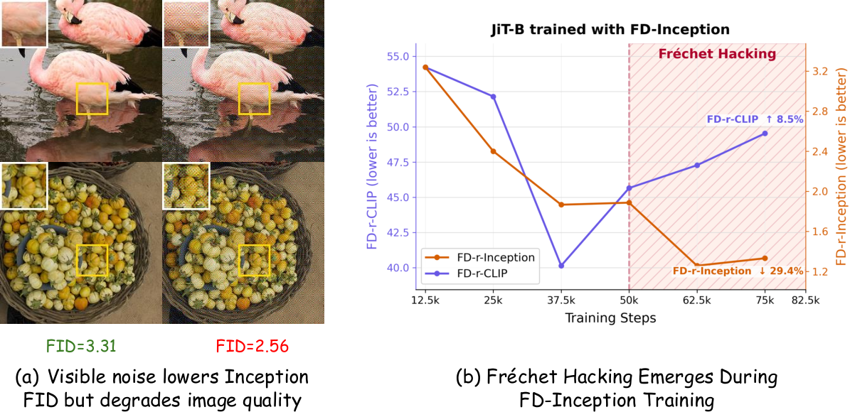
Merely adding more frozen encoders enlarges coverage but leaves the fundamental issue — the encoders do not adapt as q_\theta evolves.
Method: adversarial Fréchet distance
AdvFD complements the static FD objective with a learnable representation \psi_{\omega} that is trained adversarially. Let \mathcal{F} be the frozen encoder set (the paper uses SigLIP + MAE + Inception, “SIM”). The static term is
D_{\mathrm{static}}(p,q_\theta) = \sum_{\phi \in \mathcal{F}} \lambda_\phi D_{\mathrm{FD}}^\phi(p,q_\theta).
At iteration t, an adaptive term D_{\mathrm{adv}}(p, q_\theta; \omega_t) is added, giving
\mathcal{L}_t(\theta;\omega_t) = D_{\mathrm{static}}(p,q_\theta) + \lambda_{\mathrm{adv}} D_{\mathrm{adv}}(p,q_\theta;\omega_t).
Training alternates two steps:
- G-step: freeze \mathcal{F} and \psi_{\omega_t}; update \theta by descending \nabla_\theta \mathcal{L}_t.
- D-step: freeze \theta; update \omega to maximize D_{\mathrm{adv}}, exposing residual discrepancies missed by the fixed encoders.
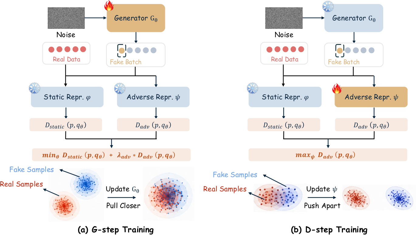
This is a GAN-like game, but the “discriminator” is a feature extractor and the payoff is a Fréchet distance on its features rather than a classification loss. The abstract notes a calibration mechanism preventing the adversarial encoder from trivially inflating the objective through feature-norm amplification (details truncated in the provided excerpt), which is essential — otherwise \omega would simply scale \psi_\omega’s outputs.
\psi_\omega is initialized from a pretrained visual encoder, so the adversary starts in a semantically meaningful space rather than a random projection, which likely stabilizes early training. The generator sees gradients only through generated samples; real samples enter only via the Fréchet statistics.
Results
Evaluation is on class-conditional ImageNet-1K at 256\times256 with JiT and pixel MeanFlow (pMF) backbones at B/L/H scales, using one-step (1-NFE) sampling and 50k generated samples per evaluation. Three metrics are reported:
- FID (Inception, in-training encoder),
- FD-r6: normalized FD averaged over six encoders (Inception, ConvNeXt, DINOv2, MAE, SigLIP, CLIP),
- FD-r3: the same average restricted to ConvNeXt, DINOv2, and CLIP — encoders not used in the SIM training loss. FD-r3 is the key transfer metric: it measures whether gains generalize outside the training feature spaces.
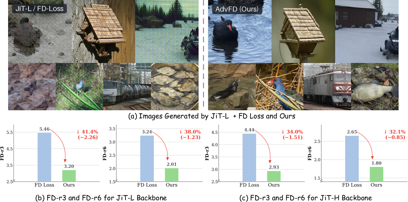
Reported relative reductions of FD-r3 / FD-r6 versus the static FD-loss baseline:
- JiT-L: 41.4% / 38.0%
- JiT-H: 34.0% / 32.1%
The larger drop on FD-r3 than FD-r6 is the point: improvements are strongest in encoders the model was not trained on, indicating the adversarial term is closing genuine distributional gaps rather than overfitting the SIM feature spaces. Qualitatively, JiT-L + AdvFD produces cleaner and more coherent 1-NFE samples than the static-FD baseline.
Limitations and open questions
- The provided excerpt truncates the calibration mechanism for \psi_\omega. Whether it is spectral normalization, feature-norm regularization, or an EMA constraint materially affects reproducibility and stability.
- Only ImageNet-1K at 256^2 with one-step generators is evaluated. Whether AdvFD improves multi-step diffusion sampling or text-to-image models at higher resolutions is untested.
- The adversarial representation adds a full encoder to the training loop, increasing compute and memory. No wall-clock comparison against expanding \mathcal{F} with additional frozen encoders is reported here.
- FD-r3 still uses fixed encoders; a sufficiently adversarial optimizer could in principle exploit blind directions in the union of SIM ∪ ConvNeXt ∪ DINOv2 ∪ CLIP. Human evaluation would strengthen the claim that the adversarial signal tracks perceptual quality.
- No comparison against classical GAN post-training (e.g., a standard discriminator on the same generator) is included in the excerpted sections, which would clarify how much of the gain comes from adversarial feature-statistic matching versus adversarial training in general.
Why this matters
Fréchet-based post-training has become a common finishing step for one-step generators, but its reliance on frozen encoders creates a well-defined Goodhart-style failure: the metric drops while quality does not. AdvFD reframes the fixed feature bank as the discriminator side of a GAN in statistic space, restoring adaptivity without abandoning the stability of distributional matching. The 30–40% FD-r3 gains on held-out encoders suggest this is the right axis on which to extend FD losses.
Source: https://arxiv.org/abs/2608.11205
Mendel Gödel Machine: Recursive Self-Improving Coding Agents via Comparative Evolution
Problem
Archive-based self-improving coding agents (Gödel-Machine-style systems: HGM, DGM) maintain a lineage tree of agent scaffolds, each stored as source code (genotype) with evaluation traces (phenotype), and iteratively rewrite themselves. The dominant self-modification primitive conditions edits on a single failure trajectory: pick a failed task \tau, feed the trace to an editor LLM, produce a new agent. This wastes the archive. A failure trace alone conflates many possible causes (bad localization, weak repair, missing validation), so single-trajectory edits are noisy diagnostics. The paper asks whether comparative evidence across the archive — same agent on multiple tasks, or different agents on the same task — yields more reliable self-edits.
Method
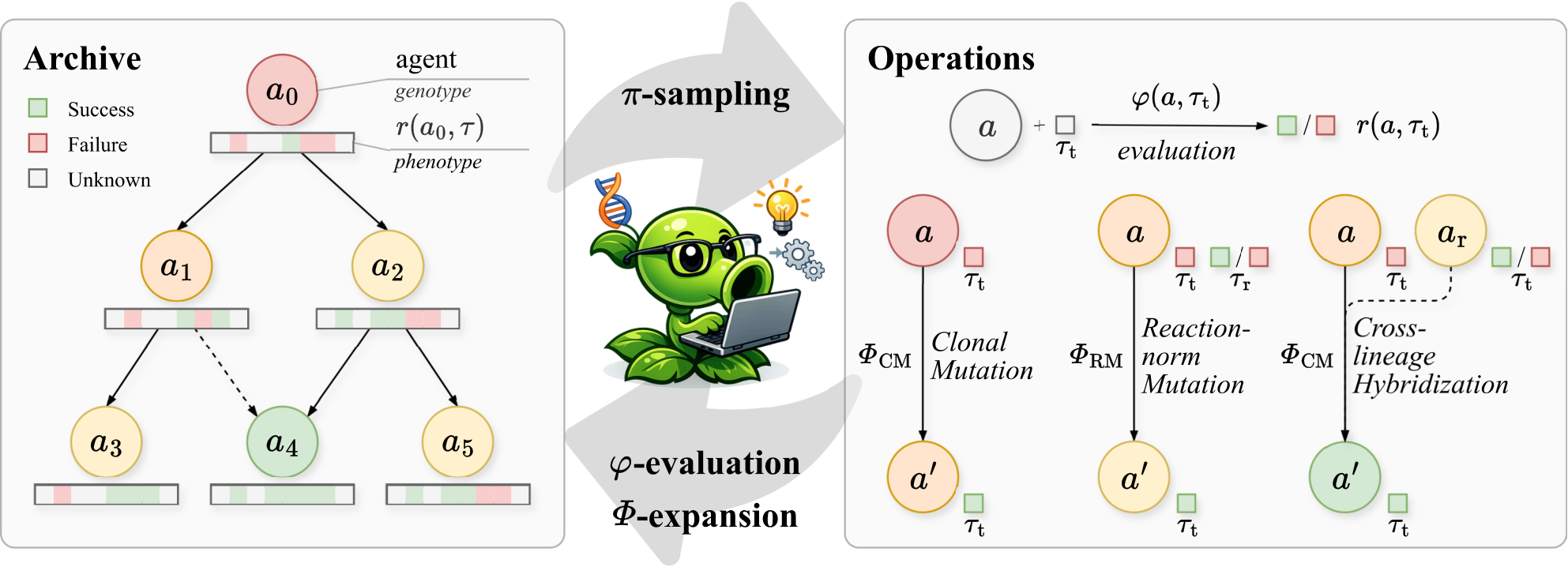
MGM keeps the standard tree-search structure (selection \pi, evaluation \varphi, expansion \Phi) but partitions \Phi into three operators keyed on the type of diagnostic evidence E:
- Clonal mutation \Phi_{\rm CM}: baseline single-agent, single-task edit. Evidence E_{\rm CM}(i,\tau)=\{(\varphi(a_i,\tau), r(a_i,\tau))\}, then a' \leftarrow \Phi_{\rm CM}(a_i, E_{\rm CM}). Used when the archive is too small to form comparisons.
- Reaction-norm mutation \Phi_{\rm RM}: same agent, multiple tasks. The editor sees the agent’s trajectory across a set of tasks simultaneously and is asked to identify the invariant weakness (e.g., recurring failure mode across environments), analogous to reading a genotype’s reaction norm across environments in quantitative genetics.
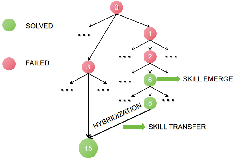
- Cross-lineage hybridization \Phi_{\rm CH}: same task, different agents. Given the selected agent’s failing trace on \tau and a reference agent from a different lineage that succeeds (or fails differently) on \tau, the editor uses the delta as a diagnostic signal to import the missing capability.
Cross-lineage hybridization requires shared diagnostic tasks across lineages; the paper picks nodes colored by outcome on such a shared task (e.g., javascript__queen-attack) to construct the reference pair.
Additive fitness landscape analysis
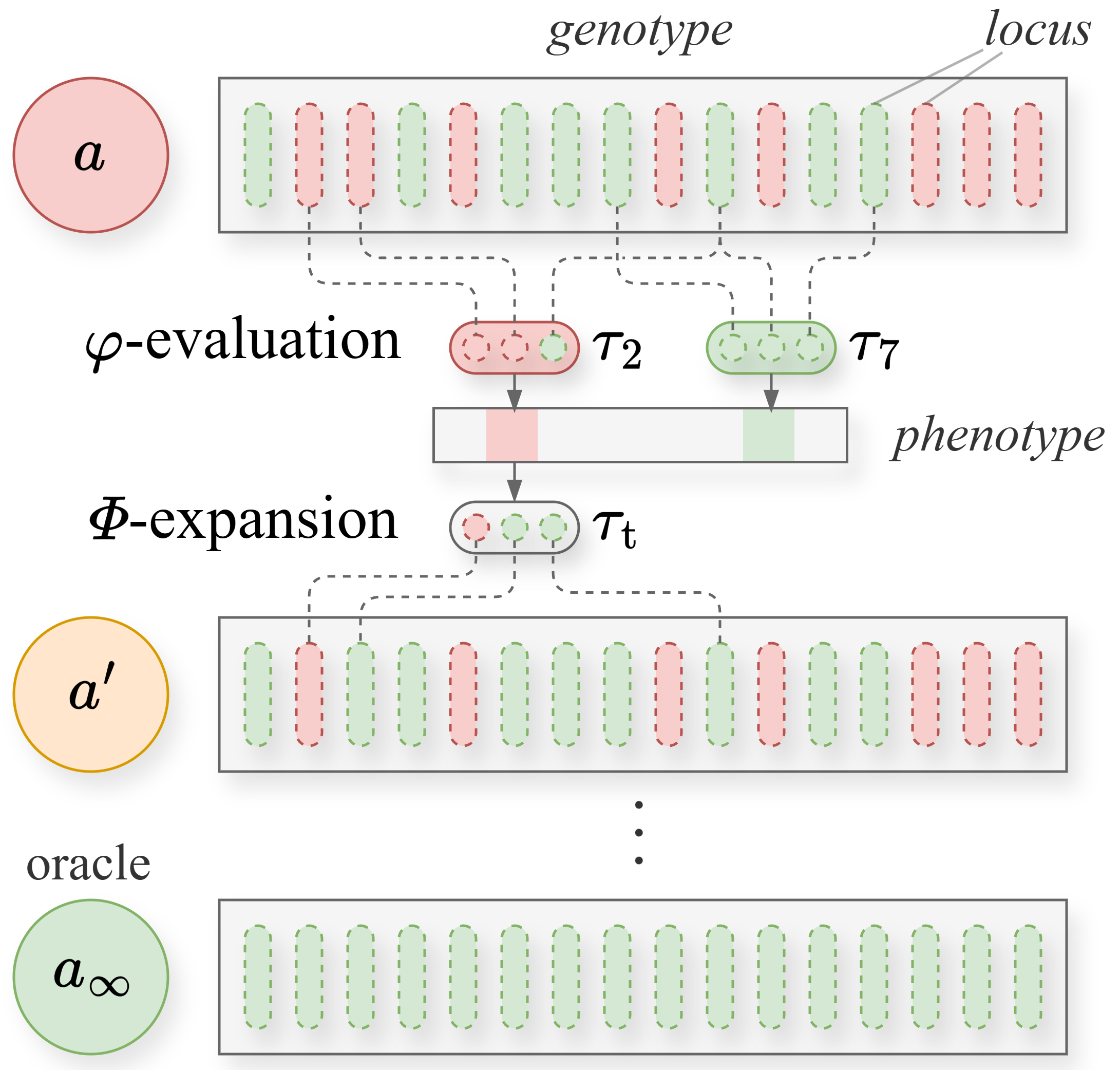
To justify the design without confounds from LLM stochasticity, the paper introduces a surrogate. Each agent has genotype \mathbf{g}\in\{0,1\}^L; oracle is \mathbf{g}^*=\mathbf{1}; distance d(\mathbf{g})=\sum_\ell \mathbf{1}[g_\ell\ne g^*_\ell]. A task \tau examines k loci R_\tau\subseteq[L] and is solved iff R_\tau\cap M(a)=\emptyset, giving
P(r=1\mid d)=\Big(\tfrac{L-d}{L}\Big)^k.
\Phi-expansion flips examined loci, correcting mismatches or corrupting correct loci with fixed probabilities. Under this model, single-trajectory clonal mutation only sees the loci in one R_\tau; reaction-norm mutation sees \bigcup_\tau R_\tau, sharpening the posterior over which loci are actually mismatched; cross-lineage hybridization further constrains it by contrasting against an agent with different M(\cdot). The paper proves and simulates that the effective fix probability rises and the expected time-to-oracle shrinks under the two comparative operators.
Results
Experiments use Qwen3.6-35B-A3B as the editor/agent backbone on SWE-bench Verified-60 and Polyglot-60, matched to HGM under a 200-\varphi-evaluation, 24-\Phi-expansion budget, starting from the same ancestor scaffold.
- SWE-bench Verified-60: initial 68.3% → HGM 73.3% (+5.0) → MGM 78.3% (+10.0). Relative improvements 7.3% vs. 14.6%.
- Polyglot-60: initial 50.8% → HGM 77.9% (+27.1) → MGM 93.2% (+42.4). Relative 53.3% vs. 83.5%.
- Average across the two: 59.6 → 75.6 (HGM) → 85.8 (MGM), i.e. +26.2 pp for MGM vs. +16.0 for HGM.
Wall-clock cost is comparable (Polyglot: HGM 44.20 h, MGM 40.14 h on 8×H100; SWE-bench: 93.02 h vs. 96.11 h). Per-operator token distributions for HGM and MGM lie in the same order of magnitude, ruling out “more tokens” as the explanation. Since evaluation and expansion counts are identical, the gain is attributable to the informativeness of comparative evidence, not a bigger search budget. The paper reports that the pattern holds on the full 225-task Polyglot benchmark.
Limitations and open questions
- Only one backbone (Qwen3.6-35B-A3B) at 200 evaluations. Behavior at longer horizons, where lineage diversity should matter more for \Phi_{\rm CH}, is not fully characterized.
- The additive fitness model assumes independent loci and uniform sampling of R_\tau; real coding capabilities are entangled and non-additive, so the theoretical fix-probability advantage is at best a directional argument.
- Cross-lineage hybridization requires overlapping diagnostic tasks and multiple lineages; the paper does not quantify how sensitive MGM is to lineage bootstrapping strategy or to selecting the reference agent.
- Test contamination on SWE-bench/Polyglot vs. pretraining data is acknowledged but not audited.
- No comparison against non-Mendelian archive-exploitation baselines (e.g., trajectory-clustering editors, contrastive prompting over k failures).
Why this matters
Self-improving agents have been bottlenecked by treating each self-edit as a reaction to one failure, ignoring the archive they are already paying to maintain. MGM shows that reusing archived trajectories as controlled comparisons — across tasks for one agent, across lineages for one task — nearly doubles the improvement per unit compute (Polyglot: +42.4 vs. +27.1 pp) without extra evaluations or token spend, suggesting the next axis of scaling for recursive self-improvement is evidence structure, not more rollouts.
Source: https://arxiv.org/abs/2608.07645
VibeLifeBench: Can Your Life Agent Be Proactive and Persistent in a Living World?
Problem
Existing agent benchmarks (τ-bench, AgentBench, WebArena, etc.) evaluate short, self-contained tool-use episodes: the user issues a request, the agent responds, the world is static in between. Real personal-assistant workloads violate all three assumptions. Tasks run for weeks; the world mutates between prompts (a flight is rescheduled, a policy changes, a phishing email arrives); many constraints (passport validity, insulin customs declaration) are never stated. An agent optimized for reactive single-turn tool use has no incentive to re-inspect state, to stay silent when appropriate, or to maintain plan coherence across a month of stages.
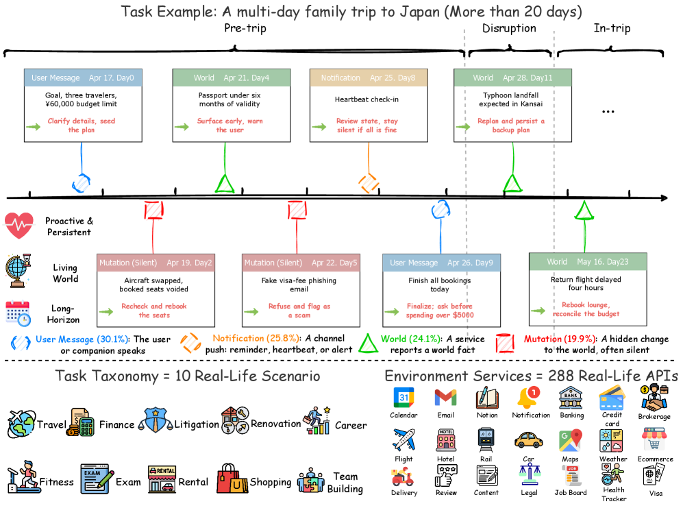
VibeLifeBench targets exactly this gap with 200 scripted multi-week tasks over 10 life domains (career, exam prep, finance, fitness, litigation, renovation, rental, shopping, team building, travel), executed against a simulated world of 22 mock services with its own clock.
Method
A task is a world with a clock, not a prompt. Within each stage, four event kinds fire: user messages, world observations, notifications, and — critically — mutations, which change world state without triggering an agent turn and without any notification. Only an agent that spontaneously re-inspects services detects them. Staying silent when nothing needs doing is scored as correct.
Grading reads only observable artifacts the agent leaves behind (bookings, drafts, messages, files) — never internal reasoning traces. Checks are organized in three tiers:
- per-stage: local outcome at the end of a stage,
- cross-stage: consistency across stages (a plan revised at day 3 must still hold at day 20),
- final: end-state correctness at task close.
Cross-stage and final checks together are 19.1% of checks but 26.8% of total weight. Each task runs three times; the report is \text{avg@3}, \text{max@3}, \text{min@3}, and within-task standard deviation \sigma (SD of a task’s scores across runs, averaged over tasks).
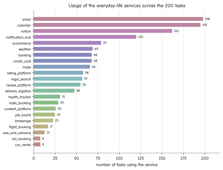
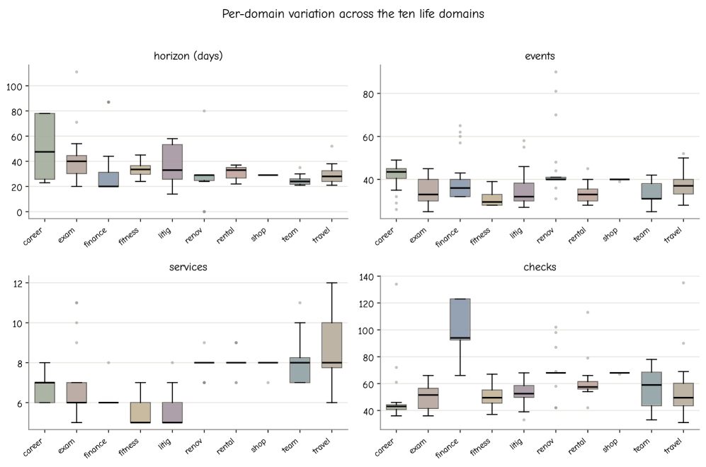
The service layer is exercised broadly but long-tailed in frequency, and domains differ in horizon, event count, service count, and check count.
Results
Seven frontier models are run with native tool-calling scaffolds at their strongest reasoning settings. Every one scores low:
| Model | avg@3 | max@3 | min@3 | \sigma | Context (M) | Tool calls | Turns |
|---|---|---|---|---|---|---|---|
| Claude Opus 5 | 32.5 | 41.2 | 23.8 | 9.8 | 30.2 | 316 | 210 |
| GPT-5.5 | 30.1 | 38.8 | 21.5 | 10.0 | 17.6 | 332 | 146 |
| Gemini 3.5 Flash | 27.5 | 35.6 | 20.1 | 8.3 | 41.2 | 243 | 227 |
| Claude Opus 4.8 | 27.5 | 34.3 | 20.3 | 7.5 | 28.8 | 228 | 111 |
| GLM-5.2 | 25.4 | 29.9 | 20.9 | 4.8 | 22.3 | 288 | 141 |
| Kimi-K2.6 | 22.6 | 27.1 | 18.4 | 4.6 | 21.8 | 231 | 166 |
| DeepSeek-V4-Pro | 21.1 | 24.7 | 17.7 | 3.7 | 13.7 | 203 | 101 |
Three findings stand out.
Ceiling is low, floor is very low. The best model reaches avg@3 = 32.5; even \text{max@3} = 41.2. Every model’s \text{min@3} \leq 23.8: at least one of three runs is close to floor for every system. All seven cluster in a 21–33 band — the inter-model spread is smaller than the distance from any of them to competence.
Unreliability is intrinsic. Within-task SD reaches 10.0 for GPT-5.5 and 9.8 for Claude Opus 5. Larger, more expensive models are not more consistent; the more reasoning-heavy Anthropic and OpenAI systems have the highest \sigma, while cheaper models (DeepSeek-V4-Pro, \sigma = 3.7) are stably mediocre. Persistence and self-consistency, the properties a long-horizon assistant needs most, are exactly where current models are weakest.
Domain competence is highly uneven. Even Claude Opus 5 ranges from 21.8 on team building to 51.1 on shopping. The easy-to-hard ordering is stable across models: shopping / travel / renovation tractable; team building / rental / exam preparation hardest. Strength on one domain does not imply broad usability.
Failure-mode analysis in Section 5 confirms the mechanism: pass rates are lowest on the cross-stage and final tiers, precisely the checks that require re-inspecting silently-mutated state and maintaining plan coherence across weeks. Fluent single-turn tool use — the capability current models are optimized for — does not compose into persistent, proactive behavior over long horizons.
Limitations and open questions
The world is a scripted simulation of 22 mock services, so results measure agent behavior under a designed distribution of silent mutations rather than the real messiness of production APIs. Grading against left-behind artifacts penalizes agents that reason correctly but fail to persist state; the flip side is that it cannot credit good judgment that produced no observable action. The benchmark also does not disentangle “the model does not know it should re-inspect” from “the scaffold does not schedule periodic re-inspection” — a targeted scaffold that polls services on a fixed cadence might close much of the gap without any change in the underlying model. Whether RL fine-tuning on silent-mutation trajectories, or memory-augmented planners with explicit re-inspection policies, close the 40-point gap to full credit is open.
Why this matters
VibeLifeBench operationalizes the difference between reactive tool-callers and agents that maintain coherent plans in a world that changes while they are not looking. The 21–33 avg@3 band across seven frontier models, together with \sigma up to 10, is a concrete measurement that current LLM agents are not yet trustworthy personal assistants on horizons longer than a session, regardless of raw model quality.
Source: https://arxiv.org/abs/2608.10875
SkillZip: Evaluation-Free Skill Compression for Self-Evolving Agents by Discovering Reusable Structure
Problem
Self-evolving agents (ACE, SkillRL, SkillClaw, SkillOpt, Memento-Skills, etc.) accumulate procedural knowledge by appending patches: warnings after tool failures, examples after format violations, new branches after rare successes. Each edit is locally sensible, but the artifact drifts into an append-only notebook rather than a maintained program. The same invariant (“never overwrite the source file”) ends up restated in the introduction, several workflow branches, and an example; the same validate–repair–verify sequence is copied with small variations. Because a loaded skill sits in the context on every invocation, this inflates prefill cost and dilutes the operative instructions.
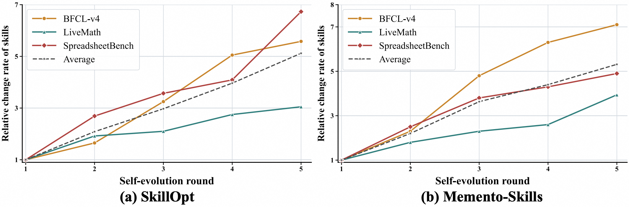
The authors document a systematic gap between textual growth and procedural growth: skill length keeps rising after genuinely new content has largely stabilized. The obvious tools do not fit. Generic prompt compressors (LLMLingua-style) decide which tokens matter for a single query, whereas a skill must remain valid for all future queries in its task class. Evaluation-guided compression (SkillReducer) uses generated tasks and rollouts to protect behavior, but this couples the compressed skill to the compression-time evaluation set and pays rollout cost. SkillZip asks whether the skill’s own structure — interface, workflow, tool/output contracts, branch guards — provides enough signal to compress without any downstream evaluation.
Method
The core observation is that a skill is a typed contract, not a flat passage.
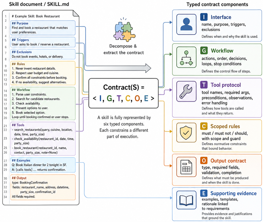
An example is removable only if every requirement it uniquely expresses is represented elsewhere in the contract. This produces the “explain once, reference many” principle: state each rule at the scope where it applies, factor repeated action sequences into shared procedures, and retain differences as explicit exceptions.
Formally, a compressed skill is a pair (\mathcal{K}, \mathcal{R}) where \mathcal{K} is a library of reusable contract elements (shared rules, workflow fragments, tool contracts, output fields, interface entries) and \mathcal{R} is a residual for unique, exceptional, or ambiguous content. SkillZip solves a typed minimum-description-length problem:
(\mathcal{K}^*,\mathcal{R}^*) = \arg\min_{(\mathcal{K},\mathcal{R})\in\mathcal{H}(S)} \big[L(\mathcal{K}) + L(\mathcal{R}\mid\mathcal{K})\big]
subject to the hard coverage constraint
a \preceq (\mathcal{K},\mathcal{R}), \quad \forall a \in \mathcal{A}_{\mathrm{req}}(S),
where \mathcal{A}_{\mathrm{req}}(S) is the set of required contract atoms extracted from the source, \mathcal{H}(S) enumerates candidate representations, and L(\cdot) is rendered token cost under the deployment tokenizer including overheads for definitions, references, and scope annotations. The constraint is what distinguishes this from prompt compression: a unique requirement cannot be dropped because it is short or because no sampled task exercises it. Compression may change how a requirement is written, never whether it is represented.
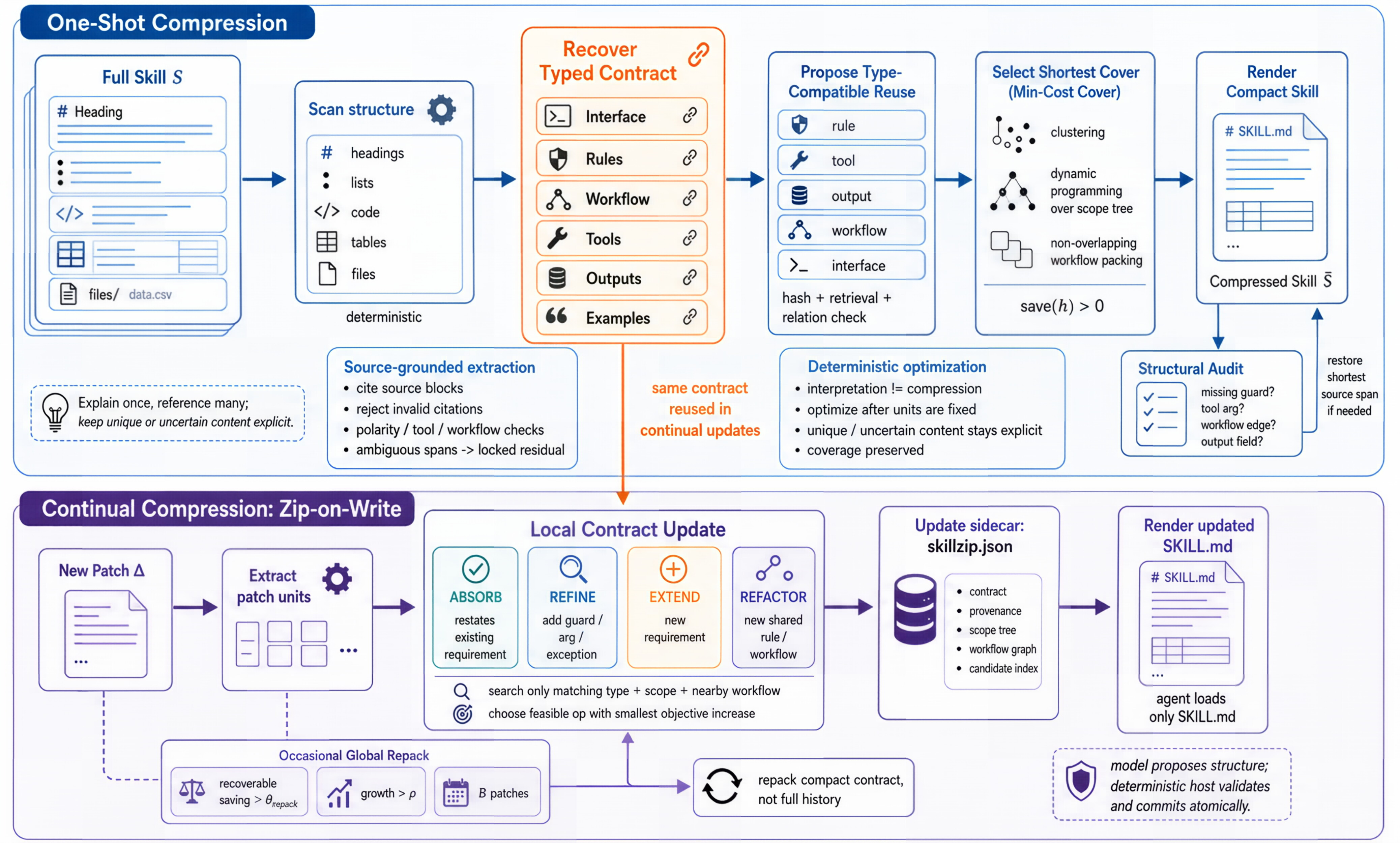
The pipeline has two modes. One-shot compression starts with a deterministic scanner over SKILL.MD that parses front matter, headings, nested lists, code blocks, tables, and file references. It copies the name/description as interface candidates, turns Markdown nesting into a preliminary scope tree, and assigns stable identifiers to source blocks. Numbered lists and temporal markers seed workflow hints. Only after this pass does a language model perform structured contract extraction, so every downstream compression decision is traceable to a specific source span. The MDL optimization then operates over this typed representation and re-renders to text.
Zip-on-Write is the continual variant: each incoming patch is compared to the affected contract neighborhood and consolidated before it becomes permanent. Occasional “repacking” runs handle reuse that only becomes visible after several patches accumulate. Ambiguous spans are kept verbatim in \mathcal{R} rather than paraphrased, making the guarantee boundary explicit.
Evaluation protocol
The experimental section defines five research questions: RQ1 quantifies skill growth during self-evolution; RQ2 studies the compression–fidelity trade-off; RQ3 measures compression cost; RQ4 tests generalization of compressed skills against baselines; RQ5 evaluates continual Zip-on-Write. Models are Qwen3.7-Max, Qwen3.6-Plus, and Kimi K2.6, spanning two capability tiers within one family and one cross-family check. Benchmarks span three procedural regimes: BFCL-v4 Web Search (multi-step retrieval with standardized tools), LiveMathematicianBench (theorem-grounded MCQ with quantifier/equivalence reasoning), and SpreadsheetBench (workbook manipulation). For each model–benchmark pair, all skill conditions share the model snapshot, scaffold, system prompt, tool definitions, interaction budget, and decoding configuration.
The provided excerpt does not include the numerical result tables. The growth-tendency figure demonstrates the qualitative RQ1 claim on SkillOpt and Memento-Skills: skill length continues to increase well after procedural novelty saturates, motivating consolidation as a distinct problem from acquisition.
Limitations and open questions
The guarantee is structural, not behavioral: SkillZip preserves every extracted contract atom, but atom extraction itself is done by an LLM after deterministic scanning, so extraction errors propagate silently. Ambiguous spans are retained verbatim, which bounds worst-case damage but also caps achievable compression. The MDL objective ranks candidate representations by rendered token cost under a fixed tokenizer; portability across backbones with different tokenizers is asserted but not shown in the provided text. It is also unclear how the method handles requirements that are only implicit in examples — e.g., a format constraint demonstrated three times but never stated — since the coverage constraint operates over extracted atoms. Finally, Zip-on-Write’s repacking schedule is described qualitatively; how often repacking should fire, and whether it can regress under adversarial patch sequences, is left open.
Why this matters
Self-evolving agent frameworks now routinely produce skills that grow monotonically in tokens while their procedural content saturates, and evaluation-guided compression re-introduces rollout cost and evaluation-set coupling that these frameworks were meant to reduce. Framing skill compression as typed MDL with hard coverage gives a clean, evaluation-free target that respects the fact that a skill is a contract, not a passage.
Source: https://arxiv.org/abs/2608.11079
Not Worth Another Token: Marginal Value Estimation for Efficient Deep Research Agents
Deep research agents built on iterative decompose-retrieve-aggregate-synthesize loops accumulate context aggressively: each subquery spawns retrievals, retrievals spawn further subqueries, and the accumulated context C_t grows superlinearly in tree depth. The marginal utility of the k-th retrieved passage, however, decays quickly — much of it is redundant, tangential, or contradictory noise that inflates synthesis cost without improving the final report. This paper asks a narrow but practical question: given a fixed pipeline (GPT-Researcher-style tree search), where along the pipeline should you spend compute filtering context, and does the choice of scoring rule matter more than the choice of stage?
Problem setup
The pipeline decomposes query Q into subqueries \mathcal{S}, iteratively selects s_t \in \mathcal{S}, retrieves C_{s_t}, and unions into accumulated context C_{t+1} = C_t \cup C_{s_t}. The objective is Lagrangian:
\max_{C_T} \mathcal{R}(C_T, Q) - \eta\,\operatorname{Cost}(C_T),
with \operatorname{Cost} combining tokens, retrieval calls, and latency. Since joint subset optimization is intractable, pruning is decomposed into three local decisions: Pre-Retrieval (drop low-value subqueries before search), Post-Retrieval (drop low-value items before they enter C_t and spawn further branches), and Pre-Synthesis (compress C_T before report generation).
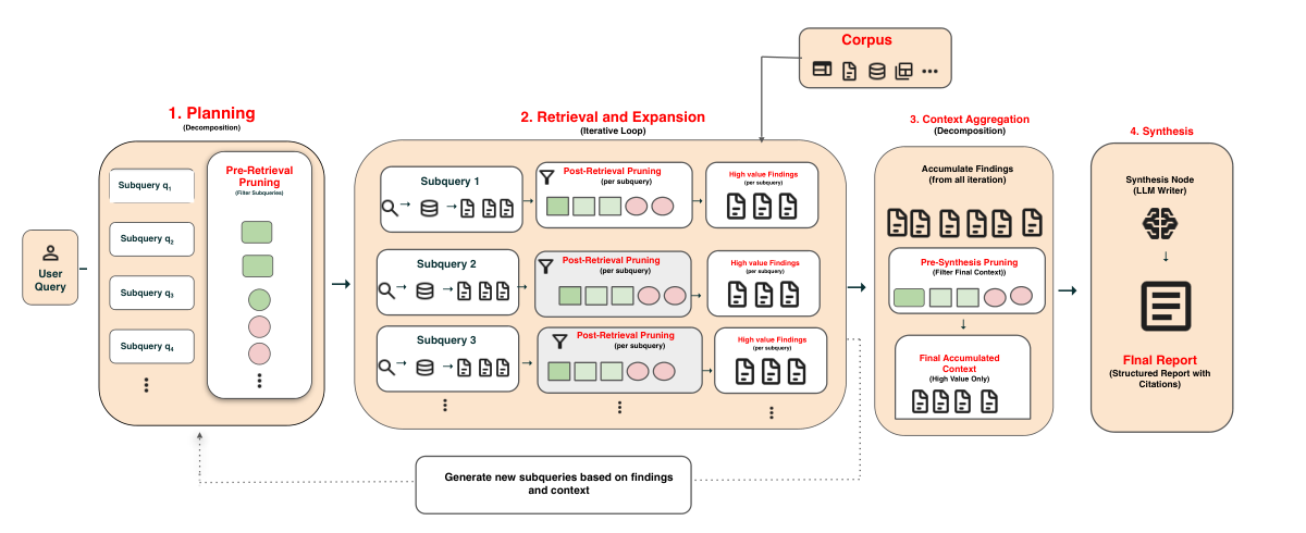
The motivating measurement makes the inefficiency concrete: the unpruned pipeline explores 29.0 nodes, consumes 375.4k tokens, and runs 3422.6s per report. Its built-in pre-synthesis trimming already drops context from 66.10 to 44.08 items (33.3% fewer items, 34.06% fewer tokens) — but this happens after retrieval and processing costs, which dominate the token bill, have already been paid.
Pruning strategies
All scoring rules operate over embeddings e(\cdot) \in \mathbb{R}^d with q = e(Q) and cosine similarity. The scalar relevance weight is w(x) = \max(\mathrm{sim}(e(x), q), 0). The paper compares:
- MMR: V_{\mathrm{MMR}}(x \mid C, Q) = \lambda\,\mathrm{sim}(e(x), q) - (1-\lambda)\max_{c \in C}\mathrm{sim}(e(x), e(c)), balancing query relevance against redundancy with retained context.
- Graph-Relevance Novelty (GRN), Coverage Diversification (CD), Semantic Coverage (SC), and a DPP kernel using \ell_2-normalized embedding Gram matrices weighted by w(x).
- Combined and Hybrid aggregates of the above.
- An LLM scorer that judges marginal value in natural language.
- A learned value model trained to predict marginal contribution.
These are evaluated at each stage and at stage combinations (Post-Retrieval only, Pre-Synthesis only, Post+Pre, and all three). Pre-Retrieval alone is excluded because its decisions are made without conditioning on retrieved content, so error sensitivity is highest.
Results
Evaluation is on 100 queries sampled from DeepResearchGym’s 1,000 Researchy Questions, with a rubric-based LLM judge for overall quality, KPR+KPC for key-point recall/coverage, and citation faithfulness.
The one-stage table sharply separates quality-optimal from efficiency-optimal configurations. Pre-Synthesis Hybrid maximizes quality at 60.68 (vs. baseline 57.83, +2.85), but tokens only drop to 332.3k and runtime remains 3834.1s — late pruning cannot recover upstream search cost. Post-Retrieval MMR is the efficiency winner: 114.6k tokens (−69.5%), 8.84 explored nodes (from 29.0), 1379.8s runtime (−59.7%), while retaining 56.62 overall quality — 97.9% of baseline. The abstract’s headline “up to 73% token reduction” comes from the more aggressive multi-stage settings.
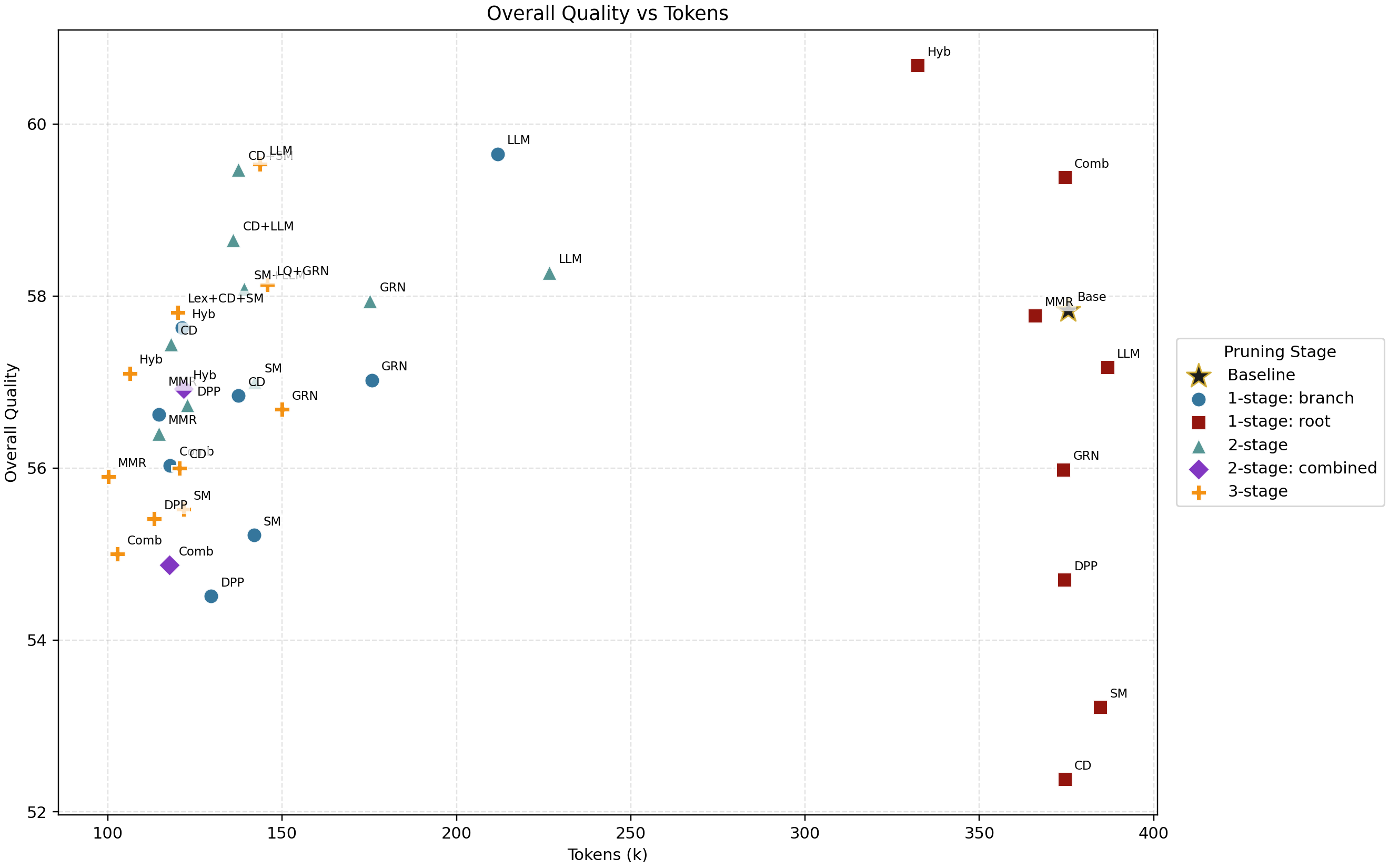
Two structural findings are worth highlighting. First, stage dominates rule: within Post-Retrieval, MMR (114.6k tokens, 56.62 quality) and the Combined heuristic (117.8k, 56.03) are near-indistinguishable, while the same rules applied at Pre-Synthesis produce fundamentally different cost profiles (node count fixed at 29.0 because search is not affected). Second, KPR+KPC (key-point recall/coverage) is more sensitive to pruning than overall quality: Post-Retrieval MMR retains 63.49 KPR+KPC vs. baseline 70.23, while GRN, CD, SC, and DPP collapse into the 41–48 range despite comparable overall quality scores. This suggests the rubric-based judge is partially compensating for missing evidence, and that key-point coverage is the stricter proxy for what pruning actually costs. Citation faithfulness stays remarkably stable (90–95) across nearly all configurations.
The LLM-based scorer, notably, is not competitive: at Post-Retrieval it consumes 211.8k tokens and 2310.7s while only reaching 59.65 quality — the scoring overhead eats most of the savings.
Limitations
The evaluation uses 100 of 1,000 available queries, so quality differences within ~1–2 points should be treated as noise. The pipeline is a single tree-structured system (GPT-Researcher); whether the “stage > rule” conclusion transfers to agentic loops with different branching factors or to non-tree architectures (e.g., graph-based aggregation, planner-critic systems) is untested. The learned value model’s training regime is under-described in the excerpts shown, and no method dominates jointly on quality, efficiency, and faithfulness — so operators must pick an \eta on the frontier explicitly. Finally, key-point recall degradation of ~7 points at aggressive settings is not negligible for domains where completeness matters (systematic reviews, legal research).
Why this matters
For anyone deploying long-horizon retrieval agents in production, this paper argues that the highest-leverage optimization is not a better relevance scorer but moving the pruning decision earlier. A trivially cheap MMR filter at Post-Retrieval delivers ~70% token savings at ~2% quality cost, whereas sophisticated LLM-based value estimation applied late is strictly dominated. The stage-aware decomposition — and the finding that the scoring rule is secondary — is a useful design prior for context management in agentic systems.
Source: https://arxiv.org/abs/2608.08389
Reference-Free Post-Training of Open Large Language Models for Multilingual Machine Translation
Problem
Post-training open LLMs for multilingual MT typically relies on parallel data with references, or on reward models trained against references. This paper asks whether a purely reference-free reward — combining QE models with a language-identification gate — can push open MT models past both strong open baselines (Seed-X, HY-MT2, TranslateGemma) and proprietary systems (Google Translate, Gemini 3 Pro, GPT-5) across 46 languages. The setting matters because reference collection is the binding constraint for scaling MT to long-tail language pairs.
Method
Starting from the SFT baseline MiLMMT-46-v0.1 at 1B, 4B, and 12B scales, the authors apply GRPO with a reference-free reward. For each source x, G candidates \{y_1,\dots,y_G\} are sampled from \pi_{\theta_{\text{old}}}, and rewards R_i are obtained by averaging two QE models, gated by a language-ID check (i.e., outputs in the wrong target language are penalized). Advantages \hat A_{i,t} are group-normalized from \{R_i\}. The training objective is the standard GRPO form:
\mathcal{J}(\theta) = \mathbb{E}_{x,\{y_i\}}\!\left[\tfrac{1}{G}\sum_{i=1}^{G}\tfrac{1}{|y_i|}\sum_{t=1}^{|y_i|}\!\Big\{\min[r_{i,t}\hat A_{i,t}, \operatorname{clip}(r_{i,t},1{-}\epsilon,1{+}\epsilon)\hat A_{i,t}] - \beta\,\mathbb{D}_{\text{KL}}(\pi_\theta\|\pi_{\text{ref}})\Big\}\right]
with token-level importance ratio r_{i,t}(\theta) = \pi_\theta(y_{i,t}|x,y_{i,<t}) / \pi_{\theta_{\text{old}}}(y_{i,t}|x,y_{i,<t}) and \pi_{\text{ref}} fixed to the SFT model.
The second component is linear checkpoint interpolation. Rather than shipping the pure RL model, the authors form MiLMMT-46-v1.0 as \alpha\cdot\theta_{\text{SFT}} + (1-\alpha)\cdot\theta_{\text{RL}}. This is motivated by the well-known SFT–RL trade-off: RL improves learned quality metrics but drifts from surface forms preferred by lexical metrics.
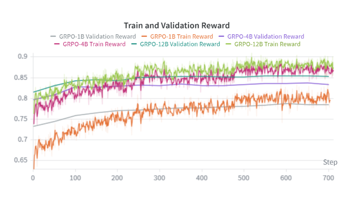
Reward curves show stable improvement across scales, with the 12B run reaching the highest validation reward as expected. The Pareto front over spBLEU and reference-based XCOMET traced by sweeping \alpha makes the interpolation motivation concrete:
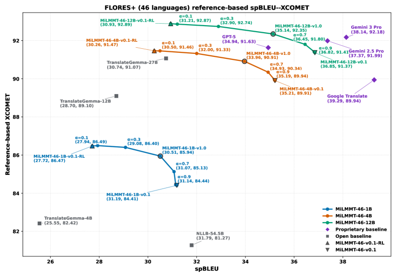
Pure RL sits at high XCOMET but reduced spBLEU; small \alpha>0 recovers most of the lexical overlap while keeping much of the quality gain.
Results
On the full 46-language block, averaged over 1B/4B/12B scales, v1.0 improves over v0.1 by:
- WMT24++ (reference-free): +2.75 XCOMET, +2.44 COMETKiwi.
- FLORES+ (averaged over en→xx, xx→en, zh→xx, xx→zh): +1.17 reference-based XCOMET, +1.41 reference-free XCOMET, +1.17 COMETKiwi, but −1.21 spBLEU.
The spBLEU drop is expected under a QE-only reward — the model is free to paraphrase away from the single reference. The consistent XCOMET and COMETKiwi gains at both reference-based and reference-free variants argue the change is genuine quality improvement, not reward hacking of a single QE model (the LID gate and QE ensemble presumably help here).
Against external systems, v1.0 leads reference-free scores on evaluated proprietary systems including Google Translate, Gemini 3 Pro, and GPT-5, and beats Seed-X, HY-MT2, and TranslateGemma on the shared-language subsets used per comparison block.
On-policy distillation
The authors ask whether the 12B v1.0 teacher can transfer gains to 1B/4B students via on-policy distillation, avoiding separate RL runs per scale. Using PG-OPD, the per-token reward is the single-sample reverse-KL estimator
r_t = -\operatorname{sg}\!\big(\log\pi_\theta(y_t|s_t) - \log\pi_\phi(y_t|s_t)\big),
optimized under the same GRPO machinery. They compare OPD alone from v0.1, OPD from v1.0, and a combined RL+OPD objective \mathcal{L}=\mathcal{L}_{\text{policy}}+\lambda\mathcal{L}_{\text{distill}}.
Results (WMT24++ ref-free XCOMET / FLORES+ spBLEU / ref-based XCOMET, avg over 46 languages):
- 1B: v1.0 = 79.01, 30.51/85.94; OPD(v0.1) = 77.67, 30.47/85.22; RL+OPD(v0.1) = 78.25, 30.49/85.67; OPD(v1.0) = 77.86, 30.39/85.42.
- 4B: v1.0 = 85.86, 33.96/90.91; OPD(v0.1) = 85.42, 34.17/90.82; RL+OPD(v0.1) = 85.85, 33.98/90.98; OPD(v1.0) = 85.37, 34.16/90.79.
At 4B, RL+OPD matches v1.0 within noise; at 1B, direct RL + interpolation is clearly better than any OPD variant. OPD reaches but does not surpass the frontier set by RL + checkpoint interpolation.
Limitations and open questions
- The reward is defined by two QE models plus an LID gate; while ensembling mitigates single-metric hacking, the evaluation also leans heavily on XCOMET/COMETKiwi. The spBLEU drop and the reliance on learned metrics both leave open whether human raters would concur, particularly for low-resource pairs where QE models are themselves weaker.
- The KL anchor \beta and interpolation weight \alpha are two knobs pointing in similar directions (staying close to SFT). The paper does not appear to disentangle them: is interpolation just a cheaper surrogate for a larger \beta?
- OPD underperforming RL+interpolation at 1B is not fully explained. Reverse-KL from a much larger teacher may be a poor training signal when the student cannot represent the teacher distribution.
- Language coverage stops at 46; behavior on truly low-resource pairs where QE models degrade is not characterized in the excerpts.
Why this matters
Reference-free post-training with a QE-ensemble reward plus SFT–RL checkpoint interpolation is a simple recipe that closes and exceeds the gap to frontier proprietary MT on learned quality metrics across 46 languages, without needing parallel references at RL time. If the QE-metric gains hold up under human evaluation, this is a practical path to scaling open MT to the long tail.
Source: https://arxiv.org/abs/2608.10812
Hacker News Signals
Stealing Reasoning Traces from Proprietary LLM APIs
The core claim: chain-of-thought reasoning traces leaking from APIs like o1/o3 can be extracted even when the provider suppresses them in the final response. The attack exploits timing side-channels and token-probability differentials. By carefully constructing prompts that force the model into a reasoning branch and then measuring latency distributions across many queries, an adversary can partially reconstruct the internal scratchpad. A second vector involves logprob probing — querying for continuation probabilities on candidate reasoning snippets to confirm or deny their presence in the suppressed trace. Neither attack requires any special API access beyond standard completions endpoints.
The threat model is realistic: providers like OpenAI sell “hidden reasoning” as a feature (users pay for compute but cannot inspect the CoT), and these traces contain intermediate conclusions, tool-call plans, and sometimes verbatim user-data echoes. Reconstructing even partial traces leaks model internals that competitors could use for distillation.
Mitigations discussed include adding calibrated noise to latency, discretizing token generation into fixed time buckets, and restricting logprob access — all of which carry throughput or utility costs. The site documents reproducible PoC code against live endpoints. The HN thread debates whether this constitutes a “vulnerability” given that providers never formally guaranteed trace confidentiality, but the practical distillation risk is real regardless of the legal framing.
Source: https://stolen-thoughts.com/
H3-metal – Native MiniMax-H3 inference for Apple Silicon
Antirez (Salvatore Sanfilippo, Redis author) published a pure-C implementation of MiniMax-H3 inference targeting Apple Silicon via Metal. H3 is a hybrid SSM architecture: it interleaves multiplicative attention layers with H3 state-space layers derived from S4, replacing the O(n^2) attention kernel with O(n) recurrent state transitions for most of the sequence budget.
The implementation bypasses llama.cpp and Metal Performance Shaders wrappers entirely, writing MSL compute kernels by hand. Key design choices: the recurrent SSM state is kept in a single persistent buffer between decode steps, eliminating the KV-cache entirely for those layers; attention layers use a tiled matmul kernel tuned for M-series unified memory bandwidth. The codebase is intentionally minimal — under 3,000 lines of C plus MSL — making it a readable reference for anyone studying SSM inference on consumer hardware.
Performance numbers in the README show competitive tokens/sec against llama.cpp on equivalent transformer models at similar parameter counts, which is notable because SSM decode is theoretically cheaper per token once the state is populated. The catch is prefill: chunked convolution for the SSM layers is less parallelizable than attention on GPU, so time-to-first-token lags for long prompts.
The project also demonstrates that MiniMax-H3 weights can be quantized to 4-bit without the numerical instability problems that plague SSM models when trained with standard post-training quantization — antirez applies a per-channel scale before quantization of the state-transition matrices.
Source: https://github.com/antirez/h3.c
Apple Silicon and macOS VMs: Faster LLM Inference with llama.cpp
This blog post from the cua project documents GPU passthrough into macOS VMs running on Apple Silicon hosts. The baseline problem: virtualization on M-series chips historically denied guest VMs access to the GPU, forcing llama.cpp inside a VM to use CPU-only paths and losing the 5-10x throughput advantage of Metal.
The solution uses Apple’s com.apple.hypervisor framework with VZVirtualMachineConfiguration and the recently stabilized VZMacGraphicsDisplayConfiguration plus VZMacOSBootLoader to expose the GPU to a virtualized macOS guest. The key finding is that with the correct entitlements and a macOS 14+ guest, llama.cpp inside the VM can call Metal and achieve throughput within roughly 15% of bare-metal, measured at ~35 tok/s for a 7B Q4 model versus ~42 tok/s native on an M3 Pro.
The practical use case is sandboxed agent execution — running an LLM-backed coding agent inside a disposable VM so it cannot trash the host filesystem — without paying a prohibitive inference latency penalty. The post details the entitlement plist required, the Virtualization framework API calls, and the llama.cpp build flags (LLAMA_METAL=1 with cross-compilation targeting the guest architecture, which is identical to host on Apple Silicon).
Limitations acknowledged: Linux guests cannot access the GPU this way; the technique is macOS-guest-only. Snapshot/restore of VM state while Metal contexts are live is unsupported and crashes.
Source: https://github.com/trycua/cua/blob/main/blog/gpu-passthrough-macos-vms.md
What’s the best programming language for coding agents?
Dan Luu’s piece applies a concrete, measurable proxy for “agent-friendliness”: token efficiency. The central argument is that since coding agents consume and emit code through LLM context windows, languages that express equivalent programs in fewer tokens are strictly cheaper to operate and fit more context. He computes token counts across languages for representative algorithmic tasks using the GPT-4o tokenizer (which is BPE-based and not language-aware).
Results are counterintuitive in places: Python’s verbose keyword syntax (def, return, self) and significant whitespace actually tokenizes worse than Lisp-family languages for many patterns. Rust tokenizes poorly due to lifetime annotations and trait bounds. Golfing languages aside, languages with terse but readable syntax — APL descendants, certain Lisp dialects — score well, though LLM fluency in those languages is low.
Luu’s secondary point is that token count correlates with error surface: more tokens means more positions where a model can hallucinate a wrong token, and autoregressive generation compounds errors. He sketches a rough model where error rate per token is constant, making total error probability 1 - (1-\epsilon)^n for n tokens — so minimizing n directly minimizes failure probability.
The piece deliberately avoids the confound that LLMs are trained on Python-heavy corpora and may be more accurate in Python despite token inefficiency. The HN thread extensively debates this tradeoff and whether fine-tuning on a compact DSL could capture both benefits.
Source: http://danluu.com/pl-tokens/
Mistral Patent for “Code implemented tool calls”
USPTO granted Mistral AI US12670045 covering the technique of encoding tool/function calls as structured code strings within the model’s text output — i.e., having the model emit something syntactically resembling a function call in a programming language rather than a JSON blob tagged with a special delimiter, and then executing that via an interpreter.
The claims are broad: independent claim 1 covers any system where an LLM generates output containing a code-formatted invocation of an external function, a runtime parses and executes it, and the result is fed back. This is essentially the mechanism used in numerous open-source frameworks (LangChain tool use, OpenAI function calling, Anthropic tool use) and arguably predated by ReAct-style prompting and Toolformer (2023, pre-Mistral filing date).
The HN discussion is heated for good reason: the prior art case looks strong. Toolformer’s arxiv preprint (Feb 2023) demonstrates exactly this mechanism. The filing date matters for determining novelty, and several commenters are pulling Mistral’s priority date to check overlap. The broader concern is that broad software patents on LLM interaction patterns create licensing risk for open-source agent frameworks even when the technique is obvious given the prior art.
From a purely technical standpoint, code-formatted tool calls have a real advantage over JSON schemas: the model’s training distribution includes far more code than JSON API specs, so token probabilities for well-formed code calls are higher, reducing malformed-output rates.
Source: https://patentsgazette.uspto.gov/week26/OG/html/1547-5/US12670045-20260630.html
llama.cpp
The llama.app domain now serves as a polished web front-end for llama.cpp, surfacing the project to non-CLI users. The HN thread is mostly about the project’s current technical state rather than the landing page. Notable recent developments discussed: GGUF format stability after the churn of the past year; the addition of speculative decoding with a small draft model reducing mean latency by 30-40% on CPU backends; and the new llama-server binary which exposes an OpenAI-compatible HTTP API with streaming, making it a drop-in local backend for any client that targets the OpenAI SDK.
On the quantization side, the Q4_K_M and Q6_K formats now dominate practical use — the K-quants apply different bit-widths to different weight classes (attention vs. FFN) based on sensitivity analysis, recovering most quality lost by naive 4-bit quantization. IQ (importance-weighted) quants go further, using per-layer Fisher information estimates to allocate bits non-uniformly, reaching near-fp16 perplexity at 3.5 bits/weight on some models.
Backend support has expanded to CUDA, Metal, Vulkan, SYCL, and CPU (with AVX-512 and ARM NEON paths). The Vulkan backend matters for AMD GPU users on Linux who previously had to use ROCm, which has historically had poor driver support outside server SKUs.
Source: https://llama.app
Show HN: Ante, a coding agent in a single binary that runs offline
Ante is a self-contained coding agent distributed as a single statically-linked binary with no runtime dependencies. The architecture embeds a small LLM (the README indicates Qwen2.5-Coder 1.5B and 7B variants via GGUF) directly into the binary using llama.cpp compiled as a static library, alongside a tool-execution harness that handles file read/write, shell execution, and a diff-apply loop.
The agent loop is a standard ReAct-style observe-reason-act cycle: the model receives a task description plus a context window containing relevant file snippets (selected by a lightweight BM25 retrieval step over the repo), emits either a tool call or a final answer, the harness executes the tool and appends results, and the cycle repeats until the model emits a stop token or a step limit is hit. All of this runs entirely offline — no API calls, no telemetry.
The single-binary distribution is achieved via a build process that quantizes the weights and packs them as a data section. Binary size for the 1.5B variant is roughly 1.1 GB. The offline constraint is the key design invariant: useful for airgapped environments, local CI, or users unwilling to send code to external APIs.
Limitations are the obvious ones from model scale: 1.5B parameters cannot reliably handle multi-file refactoring tasks that require long-range reasoning. The 7B variant helps but at 4.5 GB binary size. The HN thread discusses whether embedding weights in the binary is better than a separate model path; the counterargument is reproducibility and single-artifact deployment.
Source: https://github.com/AntigmaLabs/ante
Noteworthy New Repositories
ShawnPana/phone-harness
A harness layer for giving software agents programmatic control over a physical or emulated Android/iOS device. The core abstraction exposes a unified action space — tap, swipe, type, screenshot, back, home — over ADB (Android) and likely xcrun/simctl (iOS), so an LLM-based agent can drive real mobile UI without a custom per-app API. The design pattern is similar to OpenAI’s operator or Anthropic’s computer-use interface but scoped entirely to mobile. Practically, this means an agent receives a screenshot observation, emits a structured action, and the harness executes it and returns the next frame, enabling closed-loop mobile task automation. Useful for building mobile GUI agents, automated QA pipelines, or benchmarking multimodal models on real-world phone tasks. The thin harness design means you can slot in any agent backbone. Primary limitation: real-device control is inherently brittle across OS versions and OEM UI skins; reproducibility of experiments requires pinned emulator snapshots.
Source: https://github.com/ShawnPana/phone-harness
Kylin010/tcpfit
A TCP tuning tool that derives parameters empirically per machine rather than applying generic recipes. The central insight is that optimal TCP buffer sizes should match the actual bandwidth-delay product of the path: BDP = bandwidth \times RTT. The tool measures this directly on the host, then probes for the rate-limiter inflection point — the throughput knee where adding more buffer yields no gain — to set tcp_rmem/tcp_wmem and related kernel parameters. This avoids both under-buffering (throughput limited) and over-buffering (bufferbloat). The per-machine measurement approach is valuable in heterogeneous data-center or cloud environments where NIC speeds, kernel versions, and network topologies vary across nodes. It fills a gap between static tuning guides (which assume homogeneous hardware) and full-blown tools like netperf or iperf (which require a cooperating remote endpoint). Limitation: inflection-point detection depends on local loopback or a reachable peer, so the methodology needs clarification for WAN paths.
Source: https://github.com/Kylin010/tcpfit
starling-build/starling
A new Linux desktop environment written in Swift, comprising a custom Wayland compositor, a Swift-native shell, and a port of the Flutter widget framework to Swift (Flutter-to-Swift framework port). The compositor is built from scratch rather than wrapping wlroots, giving the project full control over the render pipeline and window management protocol extensions. Writing the shell and compositor in Swift brings memory safety without GC pauses and lets the team share language tooling across system and application layers. The Flutter-to-Swift port means existing Flutter app authors can target the desktop with a Swift backend instead of the C++ engine, potentially reducing runtime overhead and enabling tighter platform integration. First-party apps (file manager, settings, etc.) ship in the same Swift codebase, keeping the API surface consistent. This is architecturally ambitious: replacing both the compositor and application runtime simultaneously. The main risk is ecosystem fragmentation — the Swift Linux toolchain and Flutter-to-Swift binding layer are non-trivial maintenance burdens.
Source: https://github.com/starling-build/starling
guillaumemeyer/watermarks-remover
A multi-layer tool for stripping AI-origin provenance signals from text and binary files. It targets three distinct signal classes: Unicode steganography (zero-width characters, homoglyphs, variation selectors embedded in text), statistical watermarks (hooks for rewriting token distributions to defeat schemes like Kirchenbauer et al.’s green-list approach), and C2PA/EXIF/XMP metadata from raster images (PNG, JPEG), vector graphics (SVG), documents (PDF, DOCX), and markup (HTML, Markdown). The Unicode hygiene pass normalizes to a canonical form, removing covert channels that survive copy-paste. The statistical rewrite hooks are more heuristic — true statistical watermark removal without access to the detector’s secret key is an open research problem, so this layer likely applies paraphrasing or token substitution. C2PA stripping removes the cryptographic provenance chain embedded by tools like Adobe Content Credentials. Useful for privacy-conscious document pipelines, but the statistical layer’s efficacy against keyed watermarks is unverified.
Source: https://github.com/guillaumemeyer/watermarks-remover
oversecured/Samsung_Vulnerabilities
A public disclosure repository documenting 176 vulnerabilities found in Samsung preinstalled Android applications by the Oversecured static analysis service. The findings span privilege escalation via exported components with insufficient permission checks, path traversal in file providers, intent redirection, insecure deserialization, and credential leakage — all in apps that ship with elevated system or signature-level permissions and cannot be uninstalled by end users. Each entry identifies the affected package, vulnerability class, CVE where assigned, and patch status. The security research value is twofold: the sheer density of findings in a single OEM’s preinstalled surface demonstrates how large the attack surface is before a user installs anything, and the categorized dataset is useful for training static analyzers or evaluating taint-analysis tools on real-world Android code. The repository does not include exploit PoC code but provides enough detail for security engineers to reproduce and test mitigations.
Source: https://github.com/oversecured/Samsung_Vulnerabilities
denialwm/denial
A Wayland compositor written in Flutter, positioning Flutter not as an application framework running inside a compositor but as the compositor itself. The architecture places Flutter’s render tree at the root of the display server: windows from other Wayland clients are composited as Flutter widget subtrees, so window decorations, animations, and shell UI are expressed in Dart with Flutter’s animation and layout primitives. This unifies the motion model — compositor animations and app UI share the same frame scheduler and easing curves — and eliminates the impedance mismatch between shell chrome and application content seen in conventional desktops. The implementation must handle Wayland protocol handling (likely via a native plugin or FFI to libwayland), map Wayland surfaces to Flutter textures, and forward input events. Key technical risk is latency: Flutter’s raster thread and Dart GC pauses are not designed around the strict frame-deadline requirements of a display server. Compare to Starling above, which takes a similar all-in-one approach but uses Swift.
Source: https://github.com/denialwm/denial
inbjo/MirrorProxy
An all-in-one mirror acceleration proxy built around an adapter pattern. A shared proxy core handles HTTP(S) request routing, caching, and rewriting, while per-ecosystem adapters implement the protocol-specific logic needed to impersonate upstream registries: GitHub release/raw endpoints, Docker/OCI distribution API (including manifest and blob rewriting), npm, PyPI, Cargo, Go module proxy protocol (GOPROXY), Composer, and OS package mirrors. Each adapter can rewrite redirect URLs, inject authentication, and cache blobs locally, so clients configure a single internal hostname and get accelerated access to all ecosystems. This is more cohesive than running separate Nexus/Artifactory instances per ecosystem and easier to self-host than commercial proxies. The adapter abstraction makes adding new ecosystems straightforward — implement the rewrite rules and cache key scheme for the target registry protocol. Useful for air-gapped environments, corporate networks with egress restrictions, or regions with poor connectivity to npm/PyPI/DockerHub.
Source: https://github.com/inbjo/MirrorProxy
QuantumByteOSS/quantumbyte
An open-source application builder engine targeting the gap between natural-language intent and a runnable application. The stated goal is to take a high-level description and produce a working app, positioning it as an open alternative to commercial low-code/AI-app-generation platforms. The technical approach appears to combine a code-generation pipeline (LLM backend producing scaffold code) with a visual editor that lets users refine generated components, plus a runtime that executes the output. The “engine” framing suggests the core generation and execution logic is meant to be embeddable rather than purely a hosted SaaS. For ML engineers, the interesting engineering question is how the system handles the intent-to-code mapping reliably — specifically whether it uses structured intermediate representations (e.g., a component graph or DSL) between intent and code, which would make generation more controllable than raw code synthesis. The repository is early-stage; the architecture and supported output targets (web, mobile, desktop) need further documentation to assess production readiness.