Daily AI Digest — 2026-07-14
arXiv Highlights
Weak-to-Strong Generalization via Direct On-Policy Distillation
Problem
RLVR on frontier reasoning models is expensive because the target model must generate long rollouts under a sparse verifier reward, and this cost is paid once per new model. A natural shortcut is to run RL on a smaller model and reuse the result, but naive distillation from the post-RL small teacher into a stronger student is upper-bounded (and often harmed) by the teacher’s weaker base competence. This paper asks whether one can transfer the change induced by RL on a small model — the policy shift — rather than the teacher’s final policy, and thereby uplift students that already exceed the teacher.
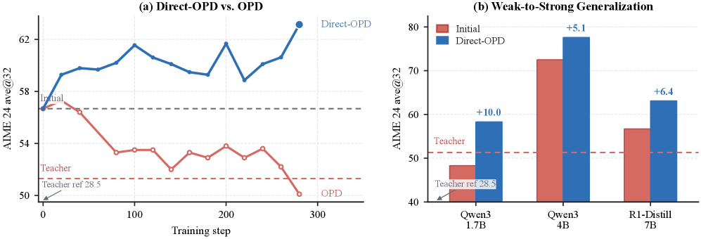
Figure 1 makes the failure mode of vanilla OPD explicit: distilling R1-Distill-7B toward the post-RL JustRL-1.5B teacher degrades the 7B student, while Direct-OPD improves it.
Method
Four policies are in play: student \pi_\theta initialized from \pi_S, and a teacher pair (\pi_{T_\text{ref}}, \pi_T) consisting of the pre-RL reference and the post-RL checkpoint. Standard on-policy distillation (OPD) samples \hat y \sim \pi_\theta(\cdot\mid x) and, on each visited prefix s_t, applies dense per-token KL to the teacher:
\mathcal{L}_\text{OPD}(\theta) = \mathbb{E}_{x,\hat y\sim\pi_\theta}\Big[\sum_t D_\text{KL}(p_t \,\|\, q_t)\Big], \quad p_t=\pi_\theta(\cdot\mid s_t),\ q_t=\pi_T(\cdot\mid s_t).
In practice teacher scores are read on the student’s top-k support S_t, yielding a signal driven by the log-ratio \log q_t(v)-\log p_t(v).
Direct-OPD keeps this on-policy, top-k interface but replaces the teacher log-probability with the RL-induced log-ratio between post-RL teacher and pre-RL reference:
r_t(v) \;=\; \log \pi_T(v\mid s_t) - \log \pi_{T_\text{ref}}(v\mid s_t).
This is a dense, per-token implicit reward that scores how much RL made the small teacher more (or less) likely to emit token v, evaluated at states the strong student itself visits. The student’s update thus climbs the RL direction in the teacher’s log-probability space, rather than matching the teacher’s absolute distribution. Because the reward is applied inside the student’s own top-k, it can re-rank actions within the student’s competence rather than dragging the student into the teacher’s mode.
Results
RQ1 (weak-to-strong transfer, Table 1a, JustRL-1.5B pair, teacher post-RL AIME24 = 51.3):
- Qwen3-1.7B: 48.3 → 58.3 on AIME24 (+10.0), 36.8 → 43.2 on AIME25 (+6.4).
- Qwen3-4B: 72.5 → 77.6 (+5.1), 65.6 → 68.8 (+3.2). The student starts above the post-RL teacher yet still gains.
- R1-Distill-7B: 56.7 → 63.1 (+6.4), 40.5 → 48.8 (+8.3).
The QuestA-Nemotron pair (different pipeline and data) yields Qwen3-1.7B 48.3 → 59.0 (+10.7) and R1-Distill-7B 56.3 → 61.2 (+4.9) on AIME24, showing the effect is not an artifact of the JustRL teacher.
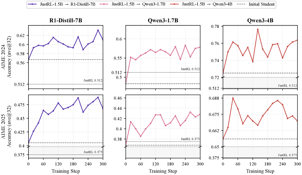
RQ2 (compute-matched comparison against direct RL on the 7B target):
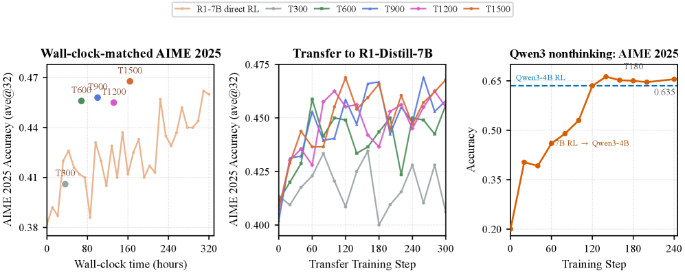
Under a shared training budget, running RL on the 1.5B and transferring via Direct-OPD reaches higher accuracy on R1-Distill-7B in shorter wall-clock than running RL directly on the 7B — the small model’s rollouts are cheap and the transfer step avoids sparse-reward exploration on the large target.
What is actually being transferred
If Direct-OPD were disguised imitation, teacher–student top-k overlap should increase. Using the standard overlap ratio |T_k^S(s_t)\cap T_k^C(s_t)|/k, the paper finds a split: the pattern-aligned R1-Distill-1.5B → 7B transfer does enter a higher-overlap regime with the post-RL teacher, but the cross-family transfers (JustRL → Qwen3, QuestA-Nemotron → R1-Distill-7B/Qwen3) do not — and overlap with the reference teacher does not rise either. Gains occur without either checkpoint being imitated in the top-k sense. This is consistent with the log-ratio r_t acting as a re-ranker over the student’s own high-probability tokens: the student climbs the RL direction while its support remains its own.
Limitations and open questions
- The teacher pair must share a tokenizer with the student for r_t to be well-defined at the token level; cross-tokenizer transfer is not addressed.
- The magnitude and sign of r_t depend on how much the small teacher’s RL run moved: a saturated or degenerate teacher pair should yield a weak or noisy reward. The paper notes needing to tune the KL coefficient across teacher–student pairs (Section 4.3), suggesting the effective learning rate on the transferred signal is not universal.
- All evidence is on math reasoning (AIME 2024/2025). Whether policy-shift transfer holds for coding, agentic tool-use, or non-verifiable domains is untested.
- The additive/compositional claim (RQ3) that multiple independently learned shifts can be stacked is asserted but not detailed in the excerpts.
- No ablation of whether r_t evaluated at T_k^S vs. T_k^T matters, nor of how far \pi_T can drift from \pi_{T_\text{ref}} before the log-ratio becomes unreliable off-support.
Why this matters
If RL improvements can be decoupled from the model that produced them and expressed as a token-level log-ratio reward, then post-training becomes a reusable artifact rather than a per-model recompute. This reframes weak-to-strong supervision away from imitation and toward transferring optimization directions, which is a cheaper and more compositional path as target models continue to scale.
Source: https://arxiv.org/abs/2607.05394
EgoSteer: A Full-Stack System Towards Steerable Dexterous Manipulation from Egocentric Videos
Problem
Dexterous VLA policies for multi-fingered hands lag behind gripper-based systems because language-aligned, action-accurate demonstration data at scale does not exist. Teleoperated dexterous datasets are small; egocentric human video is abundant but monocular, jittery, occluded, and unlabeled at the action level. EgoSteer targets end-to-end steerability — free-form instruction following across many tasks on a real dexterous bimanual robot — by treating the bottleneck as a data-and-infrastructure problem rather than an architectural one.
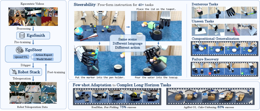
EgoSmith: turning in-the-wild egocentric video into action-labeled data
EgoSmith is a four-stage pipeline that produces 9.6K hours of curated pre-training data from 12 raw datasets at 9× the throughput of the prior SOTA HaWoR.
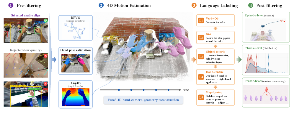
- Pre-filtering. Locomotion segments are dropped via mean optical flow on a 128×128 grid (flow magnitude correlates with head translation). YOLO-based hand detection filters occluded or bystander-contaminated frames using hand counts, scales, and coordinates.
- 4D motion estimation. They replace HaWoR’s DROID-SLAM backbone with DPVO for metric-free camera tracking plus Any4D for frame-wise metric-scale depth. Scale alignment between DPVO keyframe depths and Any4D metric depths recovers metric camera trajectories, which lift HaWoR’s camera-frame hand poses into world space. DPVO plus I/O and batching optimizations give the 9× speedup and reduce drift under rapid head motion.
- Language labeling. Qwen3.5-VL-Plus first drops 3.5% of clips lacking real manipulation, then produces a five-level coarse-to-fine instruction hierarchy per clip, providing both task-level and action-level grounding.
- Post-filtering. Coarse-to-fine outlier removal at three levels: episode (translation distribution outliers, hard rotation thresholds on head motion), chunk (spatial outliers in wrist- and finger-frame projections), and frame (hard thresholds on frame-to-frame camera/wrist/finger deltas).
Unified Robot Stack
Teleoperation uses PsiBot SynGlove-Air gloves and Vive Trackers to drive two arms (IK via mink) and two 6-DoF hands (joint mapping). The same FK/IK and control nodes serve policy inference, so training and deployment share dynamics.
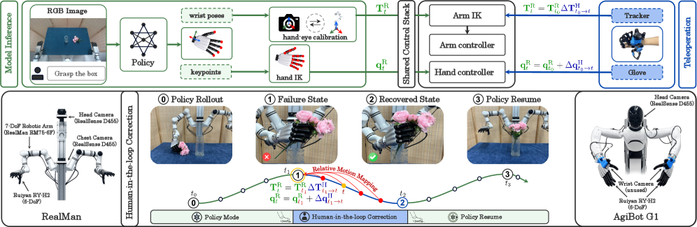
The key mechanical detail is the intervention handover. At pedal-press time t, the system snapshots robot poses \mathbf{T}^{R,i}_t, human wrist poses \mathbf{T}^{H,i}_t, and joint states \mathbf{q}^{R,i}_t, \mathbf{q}^{H,i}_t for i\in\{1,2\}. For t' \geq t, the operator’s relative motion is applied to the robot:
\mathbf{T}^{R,i}_{t'} = \mathbf{T}^{R,i}_t \,(\mathbf{T}^{H,i}_t)^{-1}\mathbf{T}^{H,i}_{t'}, \qquad \mathbf{q}^{R,i}_{t'} = \mathbf{q}^{R,i}_t + (\mathbf{q}^{H,i}_{t'} - \mathbf{q}^{H,i}_t).
This avoids state jumps at handover and yields >85% smooth-handover success. Only intervention segments are used for DAgger training. The resulting real-robot corpus is 187 hours over 193 tabletop tasks (PnP-Easy/Medium/Hard, non-prehensile, reorient, bimanual, contact-rich).
EgoSteer model
EgoSteer pairs a Qwen3-VL 2B backbone with a DiT-based action expert that jointly self-attends and cross-attends to the backbone, producing action chunks via flow matching. Episodes are unified across human and robot embodiments:
\tau = \{l, \mathbf{K}, (\mathbf{I}_t, \mathbf{D}_t, \mathbf{T}^{w2c}_t, \mathbf{s}^w_t, \mathbf{a}^w_t)_{t=0}^{N-1}\},
with \mathbf{s}^w_t, \mathbf{a}^w_t \in \mathbb{R}^{48} carrying 3D wrist translation + 6D wrist rotation + 15D fingertip keypoints for both hands. Depth is dropped; state history is transformed into the current camera frame c_t using \mathbf{T}^{w2c}_t, and actions are relative in c_t (SE(3) deltas for wrists, coordinate displacements for fingers).
Training uses conditional flow matching with training-time Real-Time Chunking (RTC): a random-delay ground-truth prefix \mathbf{a}_{\text{pre}} = \mathbf{a}_{t:t+d-1} is fed clean, and the model denoises only the suffix \tilde{\mathbf{a}}_{\text{suf}}:
\mathcal{L}_{\text{CFM}}(\pi) = \mathbb{E}_{t,\eta,\boldsymbol{\epsilon}}\left[\|\pi(\tilde{\mathbf{a}}_{\text{suf}}, \eta, \mathbf{C}_t) - (\mathbf{a}_{\text{suf}} - \boldsymbol{\epsilon})\|^2\right],
with \tilde{\mathbf{a}}_{\text{suf}} = (1-\eta)\boldsymbol{\epsilon} + \eta\,\mathbf{a}_{\text{suf}}, \eta \in [0,1], and context \mathbf{C}_t = \{l, \mathbf{K}, \mathbf{I}_{t-k+1:t}, \mathbf{s}_{t-k+1:t}, \mathbf{a}_{\text{pre}}\}. At deployment the robot executes \mathbf{a}_{\text{pre}} while the network denoises \mathbf{a}_{\text{suf}}, eliminating inference-induced execution gaps. A world-model auxiliary objective (details in the paper) is stacked on top to improve visual grounding.
Results
Pre-training: 9.6K hours at 384×384. Post-training: 187 hours of real-robot data at 640×480 (head + chest cameras). Three DAgger rounds add 3.7K trajectories / 8.3 hours of correction data across 56 tasks.
- Steerability on 32 seen tasks + 4 compositional + 4 unseen (10 trials each): overall 75% success, with 80%+ on 22 of the 40 tasks; robust adherence to instructions specifying target object, hand choice, and action, plus multi-retry failure recovery.
- Compositional generalization (novel sequences of seen primitives): 65% average success.
- Unseen tasks (novel action semantics): 62% average success.
- Long-horizon few-shot adaptation: including box folding on two embodiments, >75% success — indicating the pre-trained prior transfers with limited target data.
Limitations and open questions
The paper does not (in the shown sections) ablate world-model vs. flow-matching-only, nor quantify the contribution of DAgger separately from base post-training; those are teased under Q2/Q4 but numbers are not given in the excerpts. Depth is discarded despite being estimated, leaving the metric-scale supervision only implicit through state/action targets. Camera-frame relative actions rely on accurate \mathbf{T}^{w2c}_t at test time — degradation under rapid head motion in deployment is unaddressed. Evaluation is tabletop and short-to-medium horizon; 10 trials per task yields wide confidence intervals. Finally, the 85% handover success implies ~15% of interventions still produce discontinuities that must be filtered.
Why this matters
EgoSteer is a concrete demonstration that dexterous VLAs scale the same way gripper VLAs did: with an aggressive data pipeline, a shared teleop/inference control stack, and standard flow-matching action heads. The 9× throughput gain in 4D hand-motion curation and the relative-motion DAgger scheme are directly reusable components for any group trying to bootstrap multi-fingered manipulation from egocentric video.
Source: https://arxiv.org/abs/2607.09701
NeuroCogMap Reveals Cognitive Organization of Large Language Models
Problem
Mechanistic interpretability of LLMs has produced many isolated findings — individual circuits, features, or steering vectors — but no reproducible functional atlas that (i) organizes internal features into stable units, (ii) assigns them interpretable cognitive roles, (iii) predicts behavior under perturbation, and (iv) generalizes across models and to biological cognition. Without such an organization, characterizing failure modes like hallucination, sycophancy, bias, and refusal failure remains ad hoc. NeuroCogMap proposes a cognitive-neuroscience-style parcellation of LLM feature space — analogous to cortical atlases like Schaefer’s — to fill this gap.
Method
The construction proceeds in four stages, each mirroring a level in cognitive neuroscience.
Capability space and datasets. A capability inventory is curated from recent LLM evaluation literature, with each capability paired to an evaluation dataset. Each of the benchmarks used downstream contains roughly 2{\times}10^6 examples.
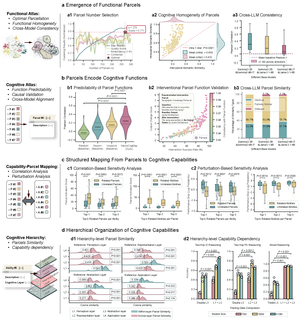
Functional atlas via SAE clustering. Sparse autoencoder features (from published SAEs for Gemma2-2B, Gemma2-9B-IT, and Llama-3.1-8B) are extracted over the capability datasets. Let a_{f,t} \in \mathbb{R} be the activation of SAE feature f on token/example t. Features are clustered by their task-evoked response profiles \{a_{f,t}\}_t into k parcels. Granularity k is chosen by a combined score:
S(k) = \alpha \cdot Q_{\text{clust}}(k) + \beta \cdot Q_{\text{desc}}(k) + \gamma \cdot (1 - R_{\text{redund}}(k))
sweeping k \in [10, 300]. The selected atlas has 270 parcels. Semantic homogeneity is validated by comparing within-parcel vs. between-parcel similarity of top-activating texts.
Cognitive atlas and capability mapping. Each parcel is assigned a natural-language cognitive description derived from its high-activation exemplars. Descriptions are validated on held-out data by predicting parcel activation from the description text (against random, per-neuron, and keyword-only baselines). Parcels are linked to capabilities using three converging signals: (a) task-evoked activation selectivity, (b) causal intervention effects on outputs, and (c) semantic consistency between description and capability.
Cognitive hierarchy. Capabilities are organized into four layers — L1 perception, L2 representation, L3 abstraction, L4 application — and validated by (i) alignment of parcel descriptions with layer-corresponding vs. non-corresponding semantic templates, and (ii) prerequisite-learning curves across Pythia model scales in controlled in-context, parametric-knowledge, and mixed reasoning conditions.
Results
Atlas quality. The 270-parcel solution shows within-parcel top-activating-text similarity substantially exceeding between-parcel similarity, indicating semantic coherence. Parcel activation is predicted from the assigned functional description far above random, per-neuron, and keyword-only baselines on held-out data (Fig. 1 b1).
Causal validity. Targeted interventions on individual parcels produce output changes consistent with the parcel’s assigned function; the joint distribution of intervention success rate and output-change score is dominated by function-consistent points (Fig. 1 b2). For parcel–capability links, perturbing related units causes larger drops in ground-truth log-probability than perturbing unrelated units, in both directions of the mapping.
Cross-model conservation. Matched parcels across Gemma2-2B, Gemma2-9B-IT, and Llama-3.1-8B show activation-pattern correlations well above random-parcel baselines, and cross-LLM function labels are classified largely as identical or partially similar rather than different (Fig. 1 a3, b3). The organization is thus partly conserved across architectures and scales.
Hierarchy validation. L1–L4 parcel descriptions align preferentially with corresponding hierarchy-layer semantic templates. In Pythia sweeps, controlled reasoning accuracy shows layered prerequisite acquisition: parametric-knowledge and in-context sub-skills emerge before mixed reasoning as scale increases, consistent with the L1→L4 ordering.
Failure-mode signatures. The framework provides distinct multi-level signatures for four canonical LLM failures. Hallucination corresponds to disruptions in representational systems — anomalous circuit connectivity among representation-layer parcels, altered parcel activation patterns, and shifted capability recruitment relative to normative responses.
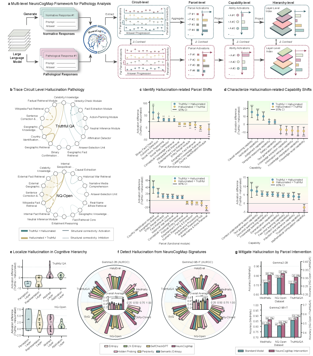
Refusal failure, sycophancy, and bias instead localize to behavioural-control systems. On AdvBench, successful-refusal vs. refusal-failure responses differ in circuit connectivity, parcel-level activation, capability activation, and hierarchy-level activation profiles, yielding an internal signature usable for detection.
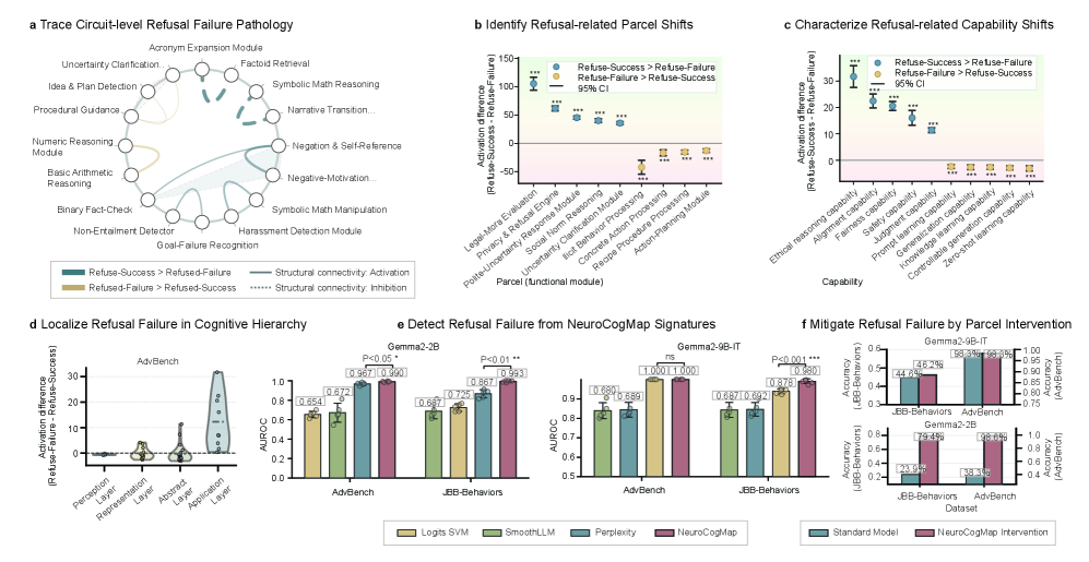
These signatures support mechanism-guided detection and targeted intervention, though the paper’s specific detection AUCs and intervention effect sizes are reported in the full results section not excerpted here.
Biological alignment. NeuroCogMap features improve prediction of human cortical responses during naturalistic language comprehension over baseline LLM-embedding encoding models (the abstract is truncated at the numerical claim).
Limitations and open questions
The atlas depends on a specific SAE decomposition; parcel identity may drift with SAE hyperparameters or training data, and the framework inherits SAE reconstruction error. The 270-parcel choice, while principled by a composite score, is a single operating point on a continuous granularity spectrum. Cross-model correspondence is “partly conserved” — exact quantitative bounds on this partial conservation across families beyond Gemma and Llama are not established. Cognitive descriptions are LLM-generated from exemplars, introducing circularity risk. Finally, the hierarchy L1–L4 is imposed by the curators; whether it emerges from unsupervised organization of parcels is not demonstrated.
Why this matters
If parcel-level functional organization is reproducible across models and causally linked to behavior, LLM failures become diagnosable at the level of specific representational or control subsystems rather than treated as monolithic emergent phenomena. This also gives a concrete substrate for LLM-to-brain comparisons that goes beyond raw embedding similarity.
Source: https://arxiv.org/abs/2607.00397
4D Human-Scene Reconstruction from Low-Overlap Captures
Problem
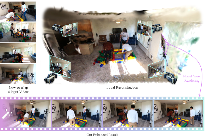
Volumetric capture pipelines assume dense, high-overlap camera rigs. In practical deployments — sports arenas, hospitals, homes — one typically has a handful of cameras (say, four) placed roughly 90^\circ apart, so adjacent views observe largely disjoint regions of the scene. Under this setup, both classical MVS (COLMAP fails outright) and recent 4D Gaussian methods (Dyn-3DGS, MonoFusion, STG) produce visible artifacts, particularly on under-observed background regions and self-occluded humans. Video diffusion priors help fill missing viewpoints but degrade human geometry consistency. StudioRecon addresses this by decoupling the two subproblems and applying an appropriate prior to each.
Method
The input is \{I_n^t\}_{n=1,t=1}^{N,T} with N\!=\!4 static, uncalibrated cameras and T\!=\!121 frames. Cameras are not pre-calibrated. The pipeline has four stages.
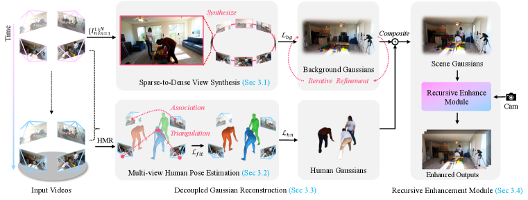
1. Sparse-to-dense view synthesis (background prior). A feed-forward 3D reconstruction model is run on the first frame across all N cameras to obtain a dense point cloud, per-view depth maps, and camera poses; these camera intrinsics/extrinsics are reused across time since cameras are static. For t>1, a monocular depth model is aligned in scale to the t=1 depths. Humans are segmented out, and background Gaussians are initialized from unmasked points with confident depth. A camera-controlled video diffusion model then synthesizes hundreds of novel viewpoints along interpolated trajectories, densifying supervision for the background Gaussians in regions no real camera observed.
2. Multi-view human pose estimation (human prior). Cross-view identity association links detections of the same subject across the sparse views, and triangulated multi-view keypoints are used to fit SMPL. This yields a robust initialization for deformable Gaussian humans, which is critical because the human reconstruction is otherwise ill-posed under 4-view sparsity with self-occlusion.
3. Decoupled Gaussian reconstruction. Backgrounds are optimized against the diffusion-synthesized dense views (where the prior is reliable and geometry is static); humans are optimized against the original real videos (where photometric fidelity is high and diffusion would inject geometric inconsistency). This split — real data where 3D geometry must be exact, synthetic data where only radiance matters — is the central design choice.
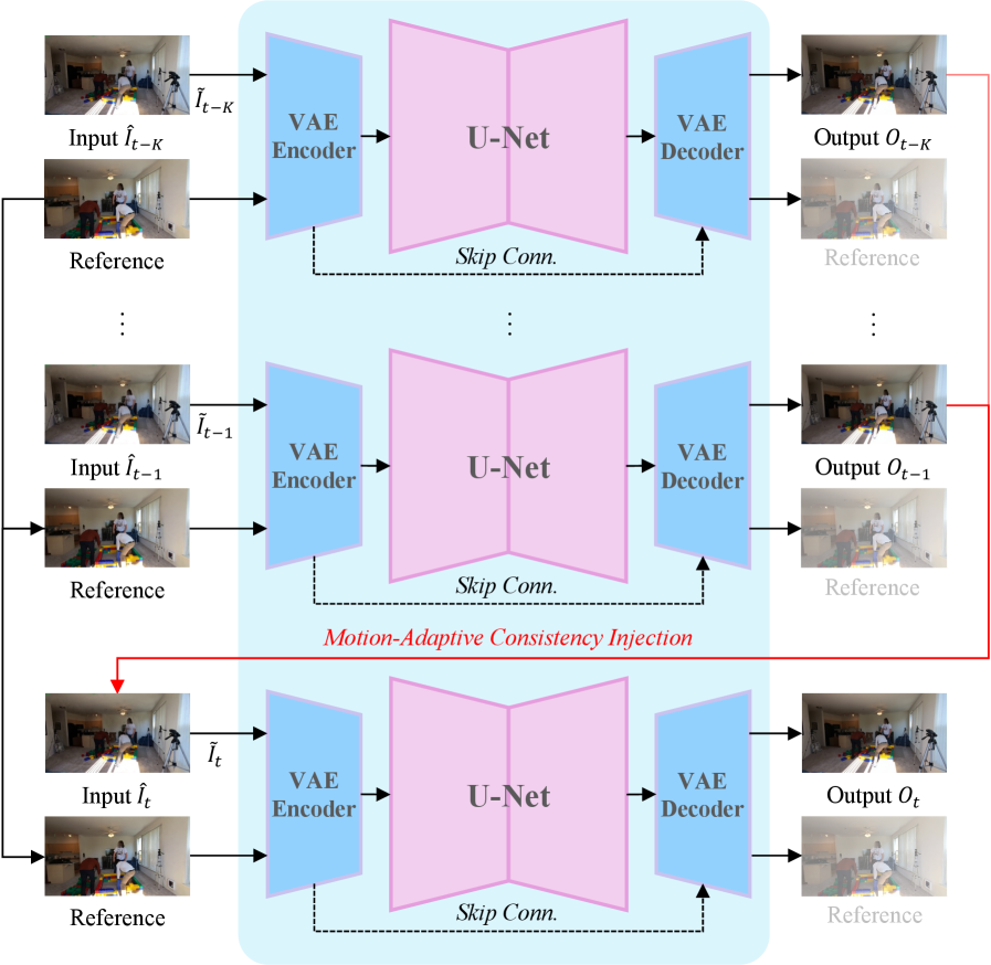
4. Recursive enhancement. The naive composite of background + human Gaussians exhibits seams and residual artifacts from mismatched supervision. A recursive enhancement module with motion-adaptive consistency injection re-renders the composite and refines it, using the temporal motion signal to gate how strongly the diffusion prior can perturb dynamic regions (which need to remain human-consistent) versus static regions (which can absorb larger refinements).
Results
Evaluation uses 4 training cameras and 4 held-out cameras at \sim 45^\circ offsets, on EgoHumans and Harmony4D (360^\circ) and Mobile Stage and SelfCap (180^\circ).
On 360^\circ scenes, StudioRecon improves PSNR over the best baseline by roughly 2–4 dB per sequence. On EgoHumans Legoassemble: 18.58 vs. 16.12 (MonoFusion); Tennis: 19.27 vs. 17.80 (STG). On Harmony4D Fencing: 22.75 vs. 20.09; Sword: 20.14 vs. 17.01; Karate: 19.90 vs. 16.94; Grappling: 19.50 vs. 16.55. LPIPS gains are more dramatic — e.g., Fencing 0.164 vs. 0.472, Sword 0.206 vs. 0.503, Karate 0.160 vs. 0.485 — reflecting the perceptual benefit of the diffusion-densified background.
On 180^\circ scenes the margin widens further: Mobile Stage Dance 21.74 vs. 16.73 PSNR (SSIM 0.575 vs. 0.336, LPIPS 0.145 vs. 0.516); SelfCap Yoga 21.63 vs. 18.72 PSNR, LPIPS 0.115 vs. 0.289. This is consistent with the hypothesis that frontal-hemisphere-only captures leave even more background unobserved, which the diffusion prior is well-positioned to fill.
Limitations and open questions
The pipeline inherits failure modes of each prior: diffusion-synthesized views can drift for large extrapolations, and SMPL-fit humans are constrained to the parametric body model, limiting fidelity for loose clothing or props. The recursive enhancement module can only mitigate — not fully hide — mismatches between the two supervision sources. The paper does not report inference/optimization cost, and generating hundreds of diffusion views per capture is presumably expensive. Robustness to feed-forward pose estimation failures is discussed only in an appendix. Finally, the approach assumes static cameras; extending sparse-to-dense synthesis to moving cameras would require conditioning the diffusion model on both target trajectories and observed motion.
Why this matters
Sparse, low-overlap multi-camera capture is the regime that practical deployments actually face, and StudioRecon shows that combining a video diffusion prior for backgrounds with a parametric-body prior for humans — kept strictly separate at optimization time — closes most of the quality gap to dense-rig methods. The decoupling recipe (real data where geometry must be exact, synthetic data where only appearance matters) is a transferable pattern for other 4D reconstruction settings.
Source: https://arxiv.org/abs/2607.09125
AdvancedMathBench: A Benchmark Suite for Advanced Mathematical Proof Generation and Verification
Problem
Contemporary math benchmarks for LLMs (MATH, AIME, olympiad sets) measure final-answer correctness on problems that admit numerical or short-form answers. This leaves two capabilities untested at the level required for research mathematics: (i) generating rigorous multi-step proofs at undergraduate-through-qualifying-exam level, and (ii) judging the validity of proof trajectories at the step level rather than only at the outcome. Prior process-level evaluation efforts either cover narrow slices (e.g., olympiad geometry, Lean-formalized subsets) or rely on coarse LLM-as-judge protocols whose agreement with expert mathematicians is unclear. AdvancedMathBench targets exactly this gap: a proof-generation benchmark (ProverBench), a proof-verification benchmark (VerifierBench), and an expert-aligned automatic verifier trained on ~2k annotated trajectories.
Construction
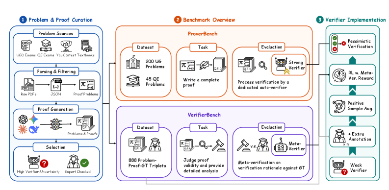
Problems are drawn from four sources chosen to span curricular breadth and difficulty: undergraduate exams from Fudan, PKU, and SJTU; doctoral qualifying exams from Stanford, UCLA, Tsinghua, and JHU; the S.-T. Yau College Student Mathematics Contest across all tracks; and textbook exercises across sub-disciplines (algebra, analysis, topology, probability, etc.). After PDF parsing and structured extraction, the pipeline discards answer-centric formats — true/false, multiple choice, fill-in-the-blank — because they admit answer-only shortcut evaluation. Only items requiring a full deductive argument are retained.
Difficulty pre-screening uses verifier uncertainty in the spirit of OPV. For each candidate problem, multiple top-tier LLMs produce proof trajectories, and Intern-S2-Preview-35B verifies each trajectory N times independently. The uncertainty is the entropy of verification outcomes,
H(p) = -\sum_{v \in \{\text{correct}, \text{incorrect}\}} p(v)\log p(v),
estimated from the verifier’s repeated calls. Problems whose generated proofs are consistently judged correct (low H, outcomes concentrated on “correct”) are dropped as too easy. At the trajectory level, trivially judged proofs are also dropped; proofs with high H — plausible but error-inducing — are retained as informative verification cases. This is a principled way to construct a benchmark whose hard problems are hard for current models, not just hard for humans.
Final expert review is performed by PhD-trained mathematicians who correct problem statements, verify or rewrite reference solutions, and prune malformed or contaminated items. The final counts: 245 problems in ProverBench (the abstract mentions 296, suggesting a version-drift between abstract and Section 3), and 888 problem–proof pairs in VerifierBench.
Automatic verifier
The verifier is trained on ~2k expert-annotated trajectories. Trajectories are diversified by generating candidates with several frontier LLMs (GPT-5.5, DeepSeek-V4-Pro, etc.) and by iterative revision from Gao et al. (2025) to produce higher-quality but still error-containing candidates. The uncertainty-based selection is reapplied to keep informative examples for annotation. The verifier outputs (1) a binary correctness verdict and (2) a fine-grained error label localizing the type of proof defect (e.g., unjustified step, incorrect application of a theorem, missing case). The paper reports strong agreement with human experts on held-out trajectories, but the exact numeric agreement is not extracted in the provided sections. VerifierBench then acts as a meta-benchmark: an LLM under test is asked to judge each of the 888 trajectories, and its judgments are compared against ground truth, quantifying whether the model can act as a proof critic in addition to a proof generator.
Experimental setup
Evaluation covers a broad frontier slate: proprietary GPT-5.5-xhigh/high, GPT-5.2, Gemini-3.1-Pro-Preview, Claude-Opus-4.8; open-source DeepSeek-V4-Pro, Qwen3.5-397B-A17B, Kimi-K2.6, GLM-5.2, gpt-oss-120b, and Intern-S2-Preview-35B. Standardized decoding: temperature 1.0, 64k max output tokens, highest reasoning effort. The provided excerpt does not include the numeric leaderboard (pass rates, verifier agreement per model), so headline generation/verification accuracies cannot be quoted from the given content. The scaffolding — 245 proof problems, 888 verification pairs, ~2k training annotations, entropy-based uncertainty selection — is what is on offer here.
Limitations and open questions
Several concerns deserve scrutiny. First, verifier-uncertainty filtering with Intern-S2-Preview-35B risks selecting against problems that this specific verifier finds hard rather than mathematically hard in general; the calibration between H and true difficulty is not established here. Second, the training set for the auto-verifier (~2k examples) is small relative to the space of proof error modes across sub-disciplines; error-type generalization to new mathematical domains (say, algebraic geometry vs. real analysis) is untested in the excerpted sections. Third, using GPT-5.5 and DeepSeek-V4-Pro both to generate training trajectories and as evaluation targets introduces a mild circularity, though the expert-annotated labels mitigate this. Fourth, the discrepancy between 296 (abstract) and 245 (Section 3) problems suggests the benchmark was still evolving; downstream users should confirm the released split. Finally, the excerpt does not report inter-annotator agreement among the PhD reviewers, which is the natural ceiling for any auto-verifier.
Why this matters
Proof-level evaluation is the natural next frontier once final-answer benchmarks saturate, and moving to graduate-qualifying-exam mathematics with an expert-aligned process verifier is a substantive step beyond olympiad answer-matching. If the auto-verifier’s expert agreement holds up, VerifierBench becomes the first sizable testbed for LLMs as proof critics — a role that matters for autoformalization, RL-from-verifier-feedback, and any future scientific reasoning agent.
Source: https://arxiv.org/abs/2607.11849
Proxy Exploration and Reusable Guidance: A Modular LLM Post-Training Paradigm via Proxy-Guided Update Signals
Problem
Post-training pipelines conflate two logically distinct steps: policy exploration (finding high-reward behaviors) and policy alignment (moving the model toward a target distribution). RL methods like GRPO do both simultaneously on the primary model, which is expensive because exploration requires many rollouts from a large policy. Distribution-matching methods like on-policy distillation (OPD) sidestep exploration but assume a pre-existing stronger teacher, imposing a strong-to-weak topology and preventing reuse of the exploration effort across models.
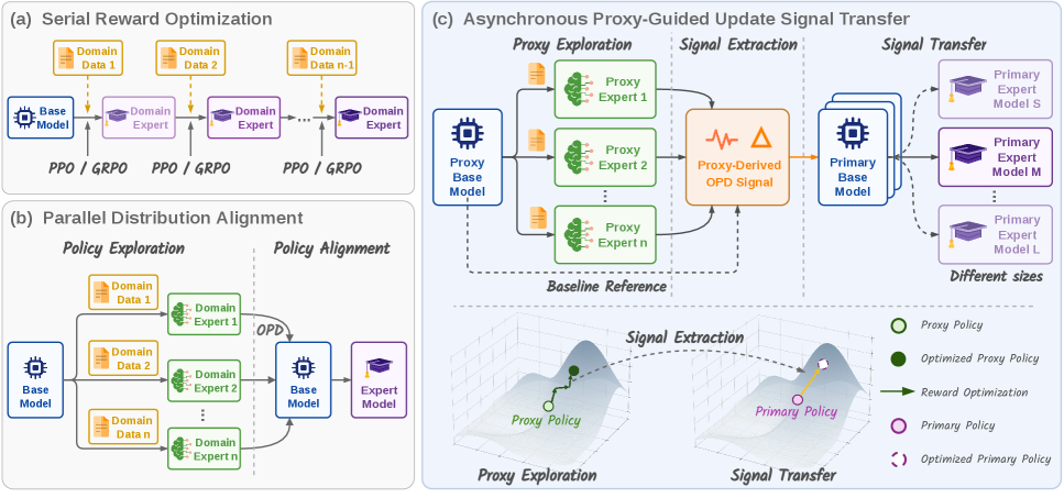
The authors argue for a third topology (panel c): explore once with a cheap proxy, then broadcast the resulting update signal asynchronously to arbitrary primary models.
Preliminary analysis: where does the useful signal come from?
Using Qwen3-1.7B, the paper compares GRPO (500 steps) against three OPD variants that align the student to the GRPO-trained teacher: standard OPD, OPD-FT (filtered trajectories, discarding groups where the student is already fully correct), and OPD-URM (token-level update-reward mask). All OPD variants converge within roughly 20 steps versus GRPO’s much longer exploratory phase, and all four converge to comparable final Mean@16 on AIME24/25.
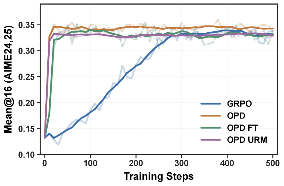
Two conclusions follow: (i) alignment itself is cheap; the expensive part is exploration; (ii) OPD is reward-agnostic — it merely matches the teacher’s distribution, so the directional signal driving improvement must be manufactured elsewhere. This motivates factoring post-training into exploration on a proxy + signal extraction + transfer.
Method: PUST
PUST defines four policies over a shared vocabulary \mathcal{V}: the initial proxy \pi_\phi, the reward-optimized proxy \pi_\phi^+ (obtained by running GRPO on the small model), the frozen primary anchor \pi_{\mathrm{ref}}, and the trainable primary \pi_\theta. At token state s_t = (x, y_{<t}), the relative update signal is the log-ratio between the two proxy states, which encodes the direction in which reward optimization moved probability mass:
\Delta_\phi(s_t) = \log \pi_\phi^+(y_t \mid s_t) - \log \pi_\phi(y_t \mid s_t).
Because the primary model lives on a different loss landscape, applying \Delta_\phi directly risks over- or under-updating. PUST calibrates the signal against the primary anchor with a coefficient \lambda, giving a target log-probability
\log \pi^\star_\theta(y_t \mid s_t) = \log \pi_{\mathrm{ref}}(y_t \mid s_t) + \lambda \, \Delta_\phi(s_t),
and drives \pi_\theta toward \pi^\star_\theta via distribution matching. The three-stage pipeline — proxy exploration, signal extraction, calibrated transfer — is illustrated below.
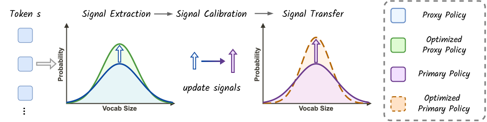
Because \Delta_\phi depends only on the proxy pair (\pi_\phi, \pi_\phi^+), it can be computed once, cached over any corpus, and reused across primary models. Exploration is decoupled from the identity and scale of the target model.
Results
Math (GRPO on DeepMath-103K, transferred to Qwen3-8B). Baseline Qwen3-8B averages 17.3 Mean@16 across AIME24/25 and HMMT25 (Feb/Nov). Directly RL-tuning Qwen3-8B (“Qwen3-4B Math (RL)” cited as the 4B RL result reaches 46.5; the 1.7B RL result 25.5). PUST with a 4B proxy transferred to 8B reaches 47.5 average (+30.2 over base), matching or exceeding on-policy RL on the 4B scale and hitting 62.5 on AIME24 vs. 58.8 for the 4B RL model. The 1.7B → 8B transfer, with \lambda = 1.5 to compensate for the smaller proxy, still yields 37.2 average (+19.9), demonstrating that a proxy roughly 5× smaller than the primary can drive substantial gains.
Code (GRPO on Eurus-RL-Code, 300 steps, 4B proxy → 8B primary). PUST reaches 60.5 average across HumanEval+, MBPP+, LiveCodeBench (+4.6 over base), versus 55.9 for the base and 56.7 for RL directly applied at 4B scale. The LCB jump is the largest: 16.7 → 25.0 (+8.3), suggesting that the extracted update direction carries reward information the primary would not easily discover under identical compute.
Calibration coefficient \lambda matters: \lambda = 1.0 suffices when proxy and primary are close in scale (4B → 8B), while \lambda = 1.5 is used for the 1.7B → 8B setting, consistent with the intuition that a weaker proxy produces a smaller-magnitude but still directionally correct \Delta_\phi that must be amplified.
Limitations and open questions
The framework assumes a shared vocabulary \mathcal{V}, so cross-family transfer (e.g., Qwen → Llama) is not addressed. Calibration is a scalar \lambda tuned per pair; a principled schedule or token-adaptive calibration would be preferable, especially since \Delta_\phi magnitudes vary across token positions and confidence levels. The reported gap between proxy-derived and primary-derived signals (Section 4.5) is acknowledged but bounded; how this gap grows with proxy-primary capability ratio, or degrades after several rounds of re-transfer, remains only partially characterized. Finally, evaluation is limited to Qwen3 at 1.7B/4B/8B scales on math and code with verifiable rewards; whether the paradigm extends to non-verifiable, preference-based rewards is untested.
Why this matters
If exploration signals are cheap to cache and broadcast, RL post-training economics change: one small-model RL run amortizes across arbitrarily many larger primaries, and update signals become a first-class artifact that can be versioned and composed. The 4B → 8B transfer matching direct 8B-scale RL is the concrete evidence that this decoupling is not merely convenient but competitive.
Source: https://arxiv.org/abs/2607.11505
LATO.2: Factorized 3D Mesh Generation with Vertex and Topology Flow
Problem
Latent flow matching has become the dominant recipe for topology-aware mesh generation (LATO, TRELLIS, etc.), but existing approaches pack vertex positions and combinatorial connectivity into a single joint latent. Continuous \mathbb{R}^3 vertex geometry and discrete adjacency \mathbf{A} \in \{0,1\}^{N\times N} have very different decoding regimes: small drift in a joint latent produces both vertex displacement and edge flips simultaneously, giving the characteristic “drifting vertices and broken surfaces” of prior work. LATO.2 argues the two signals should be factorized, and that this factorization unlocks part-wise scaling and topology-adaptive editing that a monolithic latent cannot support.
Method
The pipeline splits mesh synthesis into two VAEs and two conditional flows, all anchored to a shared coarse voxel scaffold.
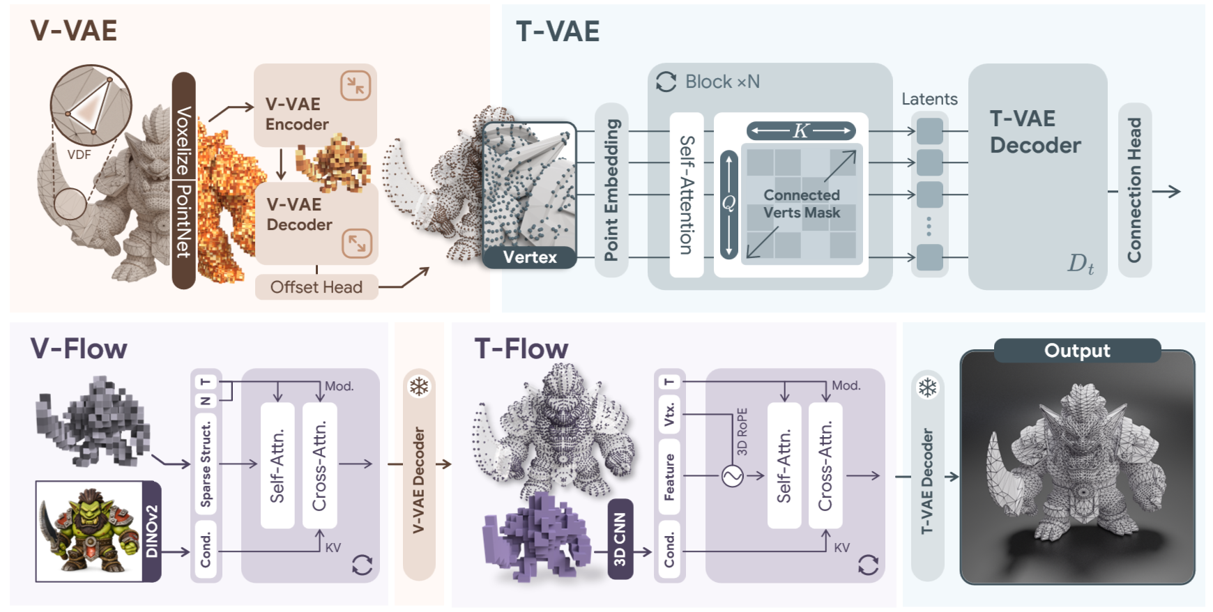
V-VAE. Rather than regressing an unordered variable-length vertex set, the encoder consumes a Vertex Displacement Field: 819,200 surface points \{\mathbf{p}_k, \mathbf{n}_k, \mathbf{d}_k\} where \mathbf{d}_k points from \mathbf{p}_k to a vertex of the face containing it. PointNet features are rasterized into a dense 1024^3 sparse voxel grid, then downsampled by sparse 3D convolutions and a sparse transformer (hidden 512, 8 heads) to a 64^3 sparse latent \mathbf{z}_\mathbf{v} with 32 channels. The decoder \mathcal{D}_\mathbf{v} inverts this via coarse-to-fine subdivision with occupancy pruning back up to 1024^3, and crucially a per-vertex sub-voxel offset head \Delta \in \mathbb{R}^3 that undoes the finest-level quantization error.
T-VAE. Given realized vertices, coordinates are discretized into K=1024 bins and Fourier-embedded to width d=768. The encoder applies adjacency-masked attention followed by full vertex attention to produce per-vertex latents with d_z=16. The decoder emits pairwise edge probabilities from an MLP classifier over vertex-feature pairs; faces are reconstructed by loop detection on the recovered adjacency.
V-Flow and T-Flow. V-Flow is a 12-block conditional Flow Matching Transformer (adapted from TRELLIS) conditioned on DINOv2 image tokens plus a target vertex-count scalar, generating \mathbf{z}_\mathbf{v}. T-Flow generates topology latents conditioned on the realized vertex set with explicit vertex positional encodings, so connectivity is drawn from p(\mathbf{z}_\mathbf{t} \mid \mathbf{V}) rather than jointly with \mathbf{V}.
Parameter counts: V-VAE 320M, V-Flow 160M, T-VAE 180M, T-Flow 240M. Training runs on 8×H100 for 4/1/7/2 days respectively; V-Flow uses effective batch 256, T-Flow uses dynamic batching over a vertex-token budget.
Factorization payoffs
Part-wise generation. Because vertices and topology are decoded independently and the vertex latent is spatially sparse, the coarse scaffold can be partitioned into part-level bounding boxes (using a controllable structure planner) and each part synthesized at full latent capacity, then merged.
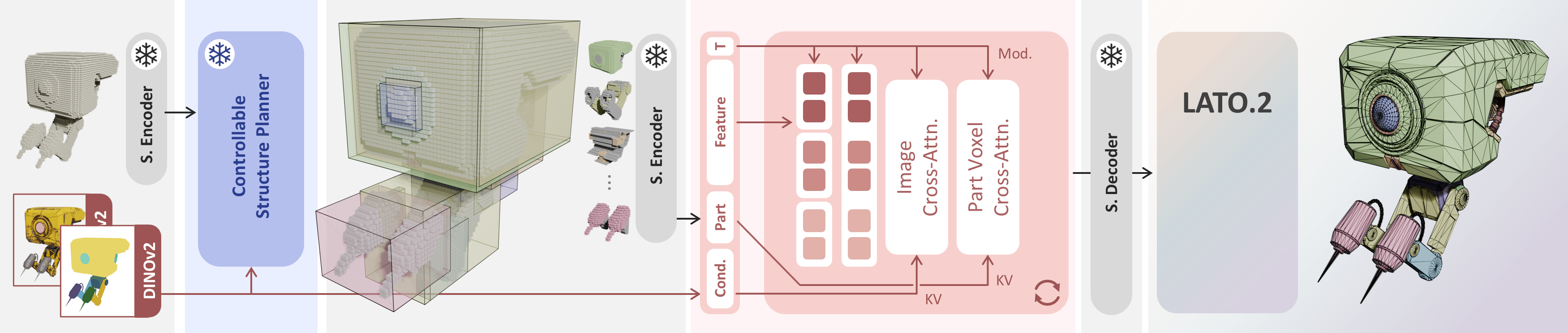
The T-Flow then closes the seams: given the union of per-part vertex sets, it synthesizes bridging faces across junctions without re-optimization. A monolithic joint latent cannot do this because per-part connectivity is entangled with global vertex positions.
Topology-adaptive editing. Because p(\mathbf{z}_\mathbf{t}\mid\mathbf{V}) is modeled explicitly, moving first-stage vertices induces a consistent re-synthesis of connectivity.
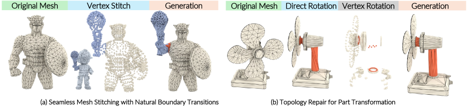
Rotating a part with connectivity held fixed causes obvious face stretching and self-intersection; passing the transformed vertices back through T-Flow yields a clean re-meshing.
Results
Training data mixes TRELLIS500K, Objaverse / Objaverse-XL, 3D-FUTURE, Toys4K, and ABO (~450K assets) with an additional 100K procedural meshes built from primitives via subdivision, twisting, warping, and composition to broaden the topological distribution.
The paper reports evaluations along four axes — reconstruction quality, conditional generation quality, topology fidelity, and ablations of the factorization. Qualitative reconstruction results (Fig. 7 in the paper) show the sub-voxel offset head materially reduces vertex localization error, with correctly recovered vertices dominating and few false positives/missing vertices; T-VAE reconstructs connectivity from ground-truth vertex sets faithfully. The excerpt provided emphasizes that ablating the offset head produces visibly larger error, and that the factorized model avoids the “broken surfaces” failure mode of joint-latent baselines.
Limitations and open questions
The excerpt does not disclose the concrete metric numbers (Chamfer distance, edge F1, watertightness rates) against baselines, so the empirical margin over joint-latent methods and autoregressive generators is not quantified here. Two structural concerns remain: (i) T-Flow’s quality is upper-bounded by V-Flow — vertex-set errors compound into implausible connectivity, and there is no closed feedback loop; (ii) discretizing vertex coordinates to K=1024 bins for T-VAE input caps positional resolution independently of the V-VAE’s sub-voxel refinement, which could limit fidelity for high-vertex-count meshes. Loop-detection-based face recovery from a predicted adjacency matrix is also known to be brittle for non-manifold or high-genus surfaces; the paper does not address behavior under such topologies.
Why this matters
Factorizing p(\mathbf{V}, \mathbf{E}) as p(\mathbf{V})\,p(\mathbf{E}\mid\mathbf{V}) is the natural generative decomposition for meshes, and LATO.2 shows it enables two capabilities — compositional part-wise scaling and post-hoc topology-consistent editing — that are structurally out of reach for joint-latent generators. This is likely the right factorization for future mesh generative stacks aimed at editable, production-grade assets.
Source: https://arxiv.org/abs/2607.10623
Hacker News Signals
Writing a bindless GPU abstraction layer
Source: https://www.kevin-gibson.com/blog/writing-a-bindless-gpu-abstraction-layer/
The post walks through building a GPU abstraction layer centered on bindless resource access — a model where shaders index into large descriptor heaps or arrays rather than binding individual resources per draw call. This matters because the traditional bind-model (OpenGL slots, DX11 constant buffer registers) imposes CPU-side overhead: every state change that rebinds a texture or buffer serializes the command stream and forces driver validation.
The core idea in modern APIs (DX12, Vulkan, Metal argument buffers) is to place all descriptors — SRVs, UAVs, samplers — into a single large heap at allocation time, then pass heap indices to shaders as push constants or root constants. Shaders declare something like Texture2D g_textures[] : register(t0, space0) and index with a runtime integer. This collapses the resource binding problem into an integer indirection, entirely on the GPU side.
The author’s abstraction layer assigns each GPU resource a persistent integer handle at creation time, analogous to a file descriptor. A ResourceManager maintains a free-list of descriptor heap slots and hands out typed handles (TextureHandle, BufferHandle). On upload, the resource is written into the heap at its assigned slot and never moved. Draw calls need only push a small constant block of resource indices rather than rebinding anything.
Key engineering details covered: managing descriptor heap fragmentation via a generational free-list (handle generation bits prevent use-after-free bugs); synchronization — because descriptor heap writes must be visible before shaders execute, requiring appropriate barriers or copy-queue synchronization; and lifetime management, where resource destruction must be deferred until all in-flight frames have retired (tracked via per-frame fence values).
The approach also simplifies multi-threading: threads can allocate and write descriptors independently since slots are disjoint. The main limitation acknowledged is that bindless requires Shader Model 5.1+ on DX12 or VK_EXT_descriptor_indexing on Vulkan, so legacy hardware support is dropped. The abstraction presented is relatively thin — one layer above DX12/Vulkan — but the handle-centric design is directly portable across both APIs.
Apple’s new SpeechAnalyzer API, benchmarked against Whisper and its predecessor
Source: https://get-inscribe.com/blog/apple-speech-api-benchmark.html
Apple’s SpeechAnalyzer API, available on-device via the Speech framework, is benchmarked here against OpenAI’s Whisper (large-v3 via a cloud endpoint) and Apple’s older SFSpeechRecognizer. The benchmark uses a corpus of real-world audio including accented speech, noisy environments, and domain-specific vocabulary — conditions that stress-test production ASR systems more than clean read-speech datasets.
The headline numbers: SpeechAnalyzer achieves roughly 5–8% WER on clean English, competitive with Whisper large-v3 and substantially better than SFSpeechRecognizer (which lands around 12–15% WER on the same clips). On noisy audio, the gap narrows — SpeechAnalyzer degrades more gracefully than the older API but still trails Whisper by 2–3 WER points in high-SNR-degradation conditions.
Latency and compute efficiency are where SpeechAnalyzer differentiates. Running entirely on-device via the Neural Engine, it processes real-time audio at roughly 0.15–0.2x real-time on an M-series chip, with no network round-trip. Cold-start latency is under 200 ms. Whisper via API incurs network latency but delivers higher accuracy on accented or multilingual speech.
The underlying architecture of SpeechAnalyzer is not publicly documented, but the benchmark authors note that it produces richer output than raw transcription: speaker diarization hints, punctuation, and confidence scores per word are returned in the result objects. SFSpeechRecognizer exposed only a flat string with limited metadata.
Practical implications: for iOS/macOS apps handling English audio in reasonably clean conditions, SpeechAnalyzer makes the Whisper API call unnecessary for most use cases, with material cost and latency savings. The remaining gap is on non-English languages — the benchmark is English-only, and SpeechAnalyzer’s multilingual support is reportedly narrower than Whisper’s 99-language coverage.
Go-Flavored Concurrency in C
Source: https://antonz.org/concurrency-in-c/
The post implements Go-style concurrency primitives — goroutines, channels, and select — in C using ucontext_t-based cooperative coroutines and POSIX threads. The goal is pedagogical: show how Go’s concurrency model maps onto lower-level primitives rather than propose a production library.
The coroutine layer uses makecontext/swapcontext to create and switch between execution contexts. Each “goroutine” gets its own stack (allocated on the heap, default 64 KB) and a ucontext_t struct. A cooperative scheduler maintains a run queue; goroutines yield explicitly or when blocked on channel operations. This is M:N scheduling with a fixed thread pool driving the scheduler loop.
Channels are implemented as a bounded ring buffer protected by a mutex, with two condition variables for full/empty states. Send blocks the sending goroutine (not the OS thread) by moving it to a wait queue and calling swapcontext back to the scheduler; receive mirrors this. The scheduler’s event loop checks for runnable goroutines and resumes them via swapcontext.
select is the hardest primitive. The implementation registers the goroutine as a waiter on all channels listed in the select, then parks. Whichever channel becomes ready first claims the goroutine via a CAS on a “selected” flag, wakes it, and the others remove it from their wait queues. This is essentially the same algorithm Go’s runtime uses, modulo the fact that Go’s implementation handles more edge cases around channel closing and starvation.
Limitations are acknowledged explicitly: no preemption (a CPU-bound goroutine starves others), no work-stealing across threads, no garbage collection for leaked goroutines, and ucontext_t is deprecated on macOS. The implementation also omits close(chan) semantics. Despite these gaps, the code is a readable ~500-line demonstration that Go’s concurrency model has a straightforward mechanical translation into C, which clarifies what the Go runtime is actually doing underneath its abstraction.
A Study of Microsoft’s Early 2026 Rollout of Claude Code and GitHub Copilot CLI
Source: https://arxiv.org/abs/2607.01418
This paper reports on an internal observational study of Microsoft engineering teams that received early access to agentic coding tools — specifically Anthropic’s Claude Code and GitHub Copilot CLI — during Q1 2026. The study methodology combines telemetry (task completion rates, session lengths, tool invocation counts) with structured developer surveys and a subset of qualitative interviews across roughly 1,000 engineers spanning backend, frontend, and infrastructure roles.
Key quantitative findings: developers using Claude Code reported a 31% reduction in time-to-first-commit on greenfield tasks, but no statistically significant improvement on bug triage tasks in large legacy codebases. Copilot CLI showed strongest uptake for repetitive shell scripting and CI configuration, with 68% of surveyed users reporting it replaced habitual StackOverflow lookups for flag syntax. Task abandonment rates — cases where the developer gave up on the agentic tool and switched to manual coding — were 22% for complex multi-file refactors, which the authors flag as a high-friction boundary case.
The study surfaces a “context cliff” failure mode: agentic sessions that exceed approximately 40 files touched or 15 sequential tool calls show sharply degraded coherence, manifesting as contradictory edits or stale file references. The authors hypothesize this is a context window management issue rather than model capability per se.
Adoption was uneven by role: infrastructure engineers showed higher tool retention at 30 days versus frontend engineers (58% vs. 39%), attributed to the higher prevalence of well-specified, idempotent tasks in infra work. Security and code review remained almost entirely human-driven despite tool availability.
Limitations: this is a single-company study with no randomized control; productivity gains could reflect novelty effects. The paper does not release raw telemetry data, citing confidentiality.
GPT-5.6
Source: https://openai.com/index/gpt-5-6/
OpenAI released GPT-5.6 as an incremental update in the GPT-5 series, positioned as a latency- and cost-optimized variant rather than a capability uplift. The model card and announcement describe it primarily as a distilled or speculative-decoding-assisted version of GPT-5, targeting interactive and agentic workloads where time-to-first-token and output throughput matter more than peak benchmark scores.
Reported characteristics: GPT-5.6 achieves roughly 2–3x the output token throughput of GPT-5 at equivalent or slightly lower per-token cost. Benchmark scores on MMLU, MATH, and HumanEval are within 1–2 percentage points of GPT-5, suggesting minimal capability regression from the optimization process. The model retains the 128K context window and tool-use capabilities of GPT-5.
OpenAI does not disclose architectural specifics — whether the throughput gains come from model distillation, quantization, speculative decoding with a draft model, or batching improvements is not stated. The framing as “5.6” rather than a separate series implies the change is deployment-level rather than a full retraining.
The API surface is unchanged from GPT-5; the model is accessible as gpt-5-6 in the chat completions and responses endpoints. Pricing is listed at a discount versus GPT-5, making it the default recommendation for production agentic pipelines where the marginal capability difference from GPT-5 is acceptable.
The announcement is thin on technical detail, consistent with OpenAI’s recent practice of releasing optimized serving variants without architecture disclosure. The HN thread reflects frustration with the naming scheme — the “x.y” versioning implies minor architectural changes but the underlying changes are opaque. Practically, the relevant signal for practitioners is the cost/latency profile, not the model number.
Migrating a production AI agent to GPT-5.6: 2.2x faster, 27% cheaper
Source: https://ploy.ai/blog/migrating-a-production-ai-agent-to-gpt-5-6
Ploy.ai documents a production migration from GPT-5 to GPT-5.6 for an agentic workflow that automates financial document processing — extracting structured data from contracts, invoices, and regulatory filings using multi-step tool calls. The post is technically substantive: they measure end-to-end pipeline latency, per-run API cost, and task accuracy across a fixed evaluation set of 500 documents labeled by humans.
Latency: median end-to-end time dropped from 18.4 seconds to 8.3 seconds per document (2.2x). The breakdown attributes most of the gain to reduced time-to-first-token and higher output throughput — intermediate tool-call responses arrive faster, which unblocks downstream steps in the agent loop earlier. For a pipeline with 6–8 sequential LLM calls, even modest per-call latency reductions compound.
Cost: $0.041 per document on GPT-5 versus $0.030 on GPT-5.6, a 27% reduction, consistent with OpenAI’s published pricing differential.
Accuracy: on their internal eval set, F1 on structured field extraction dropped from 0.924 to 0.917 — a 0.7 point regression they characterize as acceptable given the cost/latency gains. They note the regression concentrated on ambiguous date formats and multi-currency fields, and plan prompt adjustments to recover it.
The migration required no code changes beyond the model string. They did observe one behavioral difference: GPT-5.6 is more likely to emit shorter intermediate reasoning traces in chain-of-thought steps, which reduced token counts further but occasionally produced less debuggable outputs when errors occurred.
The post is a useful concrete data point: for production agentic pipelines, GPT-5.6 is a near-drop-in replacement with measurable operational wins and only minor accuracy trade-offs, at least for well-scoped extraction tasks.
Clawk: Give coding agents a disposable Linux VM, not your laptop
Source: https://github.com/clawkwork/clawk
Clawk is an open-source tool that provisions ephemeral Linux VMs for coding agent execution, isolating agent-generated shell commands, file mutations, and process spawns away from the developer’s host machine. The security model is straightforward: each agent session gets a fresh VM (via a lightweight hypervisor or container backend — the README lists firecracker and Docker as supported backends), the project directory is bind-mounted read-write into the VM, and the VM is destroyed on session exit.
The core problem it addresses is real: LLM coding agents routinely execute shell commands, install packages, and modify files as part of their operation. Running this on a developer’s laptop means a hallucinated rm -rf, a supply-chain-compromised package, or a misbehaving tool call has direct access to the host filesystem and credentials. Clawk interposes a VM boundary at low overhead — Firecracker VMs boot in ~125 ms and have ~5 MB memory overhead per VM according to the AWS Firecracker paper, making per-session isolation practical.
The implementation wraps agent invocation (currently Claude Code and a generic --cmd passthrough) to redirect execution into the VM via SSH or virtiofs. The project directory sync uses a file-watcher to propagate changes back to the host after session completion, so the developer sees final outputs without having run anything locally.
Limitations: the bind-mount-back approach means a destructive agent action inside the VM could still propagate to the host if the developer accepts the sync. The tool doesn’t currently snapshot VM state mid-session for rollback, which would be useful for multi-step agentic tasks that go wrong partway through. Network isolation inside the VM is configurable but not enforced by default, leaving exfiltration possible. The Firecracker backend requires KVM, so macOS users fall back to Docker, which provides weaker isolation guarantees.
YouTrackDB: a general-use object-oriented graph database
Source: https://github.com/JetBrains/youtrackdb
JetBrains has open-sourced YouTrackDB, the database engine that underpins YouTrack, their issue tracker. It is a fork of OrientDB — a JVM-based multi-model database supporting documents, graphs, and objects under a unified query layer. The repo positions it as a general-purpose database rather than a YouTrack-specific artifact.
The data model follows OrientDB’s design: every record is a document with a schema class, classes participate in inheritance hierarchies (hence “object-oriented”), and edges between records are first-class schema objects rather than implicit joins. This allows graph traversals to be expressed without join tables: SELECT expand(out('Blocks')) FROM Issue WHERE id = 1 returns linked issues directly. The query language is SQL-extended with graph-specific functions (out(), in(), both(), traversal depth operators).
Storage is a custom page-based engine with MVCC for transaction isolation. The WAL-based durability layer and B-tree indexes are inherited from OrientDB. YouTrackDB’s changes over OrientDB appear to include stability fixes, modernized Java dependency management, removal of deprecated OrientDB features (the enterprise clustering layer is stripped), and an updated licensing model (Apache 2.0).
Performance characteristics: OrientDB’s graph traversal performance is generally competitive with Neo4j on shallow traversals but degrades on deep or dense graphs due to in-memory adjacency list representation. Document query performance is comparable to MongoDB for small-to-medium collections but the JVM overhead and single-writer transaction model limit write throughput under concurrency.
The main interest here is provenance: a production database engine that has run at scale inside a commercial product is now open source, which provides some confidence that the edge cases have been exercised. The open question is whether JetBrains intends to actively maintain and develop YouTrackDB as a standalone product or whether this is primarily a compliance or community-goodwill release.
Noteworthy New Repositories
synthetic-sciences/openscience
An open-source AI workbench aimed at the full scientific research lifecycle: literature review, hypothesis generation, experiment design, and result interpretation. The project positions itself as a unified interface where researchers can chain LLM-backed agents against domain-specific tools (literature APIs, simulation runners, data analysis pipelines) without stitching together separate services. Under the hood it appears to follow a tool-calling agent architecture where each research primitive (search, summarize, critique, generate protocol) is a discrete callable, composable into workflows. The design emphasis is on reproducibility: workflows are serializable, so an experiment pipeline can be version-controlled and re-run. For a PhD-level user the appeal is clear — existing lab tooling is fragmented, and a single workspace that keeps provenance across LLM calls, retrieved papers, and generated artifacts reduces the bookkeeping overhead that currently falls on the researcher. It is local-deployable, which matters for unpublished data. Early-stage, so coverage of domain-specific tools is uneven, but the architecture is extensible enough to integrate custom data sources. Worth watching if you work at the intersection of ML and wet-lab or computational science.
Source: https://github.com/synthetic-sciences/openscience
linxidnju/OpenTag
A channel-native agent gateway that runs inside Slack and routes thread conversations to backend agents — Claude Code, Codex, OpenCode, Docker containers, arbitrary HTTP endpoints, or custom CLI processes. The architecture is a dispatcher: incoming Slack events are matched against routing policies (configurable per channel or per tag), dispatched to the appropriate agent backend, and responses are posted back into the originating thread. Notable engineering features include an approval workflow (a human must confirm before certain agent actions execute), persistent memory across sessions, and a structured audit log of every dispatch and response. Artifacts produced by agents (code patches, files, command output) are stored and linked in-thread. For teams already living in Slack, this avoids the context-switch to a separate coding assistant UI. The policy layer is the technically interesting piece: it lets operators enforce which agents can run in which channels, with what permissions — relevant for organizations that want LLM-assisted automation but need an audit trail. Compared to raw Slack bot integrations, OpenTag adds the routing logic, memory, and approval gates that make multi-agent Slack usage tractable at team scale.
Source: https://github.com/linxidnju/OpenTag
ibrahimqureshae/mdflux
A local-first desktop application that converts documents — including scanned PDFs — into clean Markdown suitable for feeding downstream LLM pipelines. The core technical argument is token efficiency: vision models processing raw PDF pages consume substantially more tokens than a well-extracted Markdown representation of the same content, and for large document batches that cost difference compounds quickly. MDFlux handles the extraction pipeline locally (OCR on scanned pages, structure detection, heading and table normalization) without sending content to an external API. It supports batch processing of entire folders, making it practical for research corpora or documentation libraries. The Markdown output targets AI consumption specifically: tables are normalized, extraneous formatting artifacts are stripped, and structure is preserved at the semantic level rather than the visual one. For practitioners who need to RAG over proprietary documents or feed large document sets to LLMs, the offline-first design matters for data privacy. Compared to cloud-based document parsers (AWS Textract, Azure Document Intelligence), MDFlux trades raw accuracy on complex layouts for zero data egress and no per-page billing. A reasonable trade-off for bulk preprocessing of internal documents.
Source: https://github.com/ibrahimqureshae/mdflux
jmerelnyc/Talos
A GPU worker client that participates in the Talos distributed inference network. The client pairs with a Talos account, opens a persistent WebSocket connection to the network coordinator, and serves open-model inference jobs dispatched from the network — effectively contributing idle GPU cycles in exchange for payout tied to measured uptime and completed requests. The architecture is straightforward: the WebSocket channel carries job payloads (prompt + sampling parameters), the client runs local inference (presumably via a bundled or user-supplied model runtime), and returns completions back over the same channel. Uptime reporting feeds a reputation or payout calculation on the network side. This sits in the decentralized inference category alongside Petals and similar projects, but with an explicit economic incentive layer rather than pure cooperative sharing. Technically relevant questions include how the network handles adversarial workers returning garbage completions, and whether there is any cryptographic verification of output — the repository description does not make this clear. For someone with spare GPU capacity running open models anyway, the integration cost is low. For the network to be useful as an inference endpoint, the latency characteristics of the WebSocket dispatch round-trip need to be competitive with direct serving.
Source: https://github.com/jmerelnyc/Talos
Sahir619/fable-method
A distillation of the alleged internal workflow of Claude’s “Fable” configuration into a model-agnostic prompting and scaffolding framework structured around three phases: Think, Act, Prove. The think phase handles decomposition and planning; act handles tool invocation or generation; prove handles self-evaluation against a bundled eval suite that checks whether the output satisfies the original intent. The project’s value proposition is that this loop — which mirrors standard ReAct/chain-of-thought patterns but with an explicit verification gate — can be instantiated on any instruction-following model, not just Claude. The eval component is the technically interesting piece: it operationalizes “keeping the method honest” by running automated checks on outputs rather than relying solely on the model’s self-reported confidence. For practitioners building agent pipelines, a bundled eval harness that travels with the prompting methodology reduces the gap between prompt engineering and measurable correctness. The framework is early-stage and the “Fable 5” provenance is unverified, so treat the architectural claims with skepticism. Still, the Think/Act/Prove loop with an attached eval is a practical pattern worth examining independently of its claimed origin.
Source: https://github.com/Sahir619/fable-method
Derssa/Torollo
An interactive visual playground for learning system design and networking concepts, running entirely in the browser with no external dependencies. Users construct system diagrams — services, load balancers, queues, databases, CDN nodes — and the playground simulates traffic flows, failure scenarios, and scaling events visually. The local-first constraint means the simulation engine runs client-side, which limits fidelity but eliminates any server round-trip for interaction. Technically the project is a graph-based simulation: nodes represent services with configurable properties (latency, throughput, failure rate), edges represent network paths, and a discrete-event simulator animates request propagation and queuing behavior. This is useful as a teaching tool precisely because it makes latency and failure dynamics legible — watching a single point of failure cascade is more instructive than reading about it. Compared to tools like Excalidraw or Lucidchart for system diagrams, Torollo adds the behavioral simulation layer. Compared to full network simulators (GNS3, NS-3), it sacrifices accuracy for immediacy and zero installation overhead. The target audience is engineers learning distributed systems patterns rather than network researchers needing protocol-level fidelity.
Source: https://github.com/Derssa/Torollo
eli-labz/Godcoder
A local-first desktop coding agent that uses a user-supplied LLM API key (any provider) and keeps all code on-device, with the model provider as the only external data recipient. The notable architectural claim is that the agent builds its own test harness — referred to as a “Harness” — dynamically, meaning it generates the scaffolding needed to verify its own outputs rather than relying on a pre-existing test suite. This mirrors the self-play evaluation patterns seen in research coding agents (SWE-bench solvers, etc.) but packaged as a desktop application for everyday use. The bring-your-own-key model means no intermediary sees the codebase, which matters for proprietary code. The agent architecture presumably follows a standard loop: parse task, generate code, run harness, inspect output, iterate. The self-generated harness is the differentiating claim: if it works robustly, it reduces the setup burden of having a test suite before the agent can operate reliably. Whether the generated harnesses are actually meaningful (testing the right invariants rather than trivially passing) is the critical open question. Worth evaluating empirically against a fixed benchmark before committing to it for production-adjacent work.
Source: https://github.com/eli-labz/Godcoder
jaredrhod/ai-memory-vault
A system for giving LLM assistants persistent, structured memory using an Obsidian vault as the storage backend — no vector database, no embedding index, just Markdown files with a defined schema. The architecture relies on the fact that modern LLMs with large context windows can reason over a moderate-sized Markdown document set directly, bypassing the retrieval step that RAG systems require. Memory is organized into typed notes (entities, events, preferences, open questions) with internal links following Obsidian’s [[wikilink]] convention, enabling graph traversal via plain text. Templates define the schema for each memory type, and the system includes prompting conventions that instruct the model to read, update, and create notes as part of its normal operation. The practical advantage over vector-DB-backed memory systems is zero infrastructure: Obsidian is already a common knowledge management tool, the files are human-readable and editable, and there is no embedding pipeline to maintain or drift to manage. The limitation is scale — this approach degrades as vault size grows beyond what fits in context, and there is no semantic search fallback. For personal-scale AI assistants with bounded memory requirements, the simplicity trade-off is reasonable.