Daily AI Digest — 2026-07-01
arXiv Highlights
Orca: The World is in Your Mind
Orca proposes a “world foundation model” that unifies understanding, prediction, and action under a single objective: next-state prediction in a learned latent space. Rather than committing to next-token (LLMs), next-frame (video models), or next-action (policies) prediction, Orca treats all of these as readouts from a shared latent that models state transitions. The pitch is architectural: freeze the backbone after pre-training and attach lightweight modality-specific decoders for text, image, and action.
Formulation
Given multimodal signals \mathcal{X}=\{X^m\}_{m\in\mathcal{M}}, an encoder produces a latent state \mathcal{S}=f_\theta(\mathcal{X}). State evolution is modeled bidirectionally under implicit dynamics z_t (physical laws, object properties, scene forces) and explicit conditions c_t (instructions, events):
S_{t+\Delta}\sim p_\Theta(S_{t+\Delta}\mid S_t, z_t, c_t),\quad \Delta\in\mathbb{Z}_{\neq 0}.
Both \Delta>0 (forward prediction) and \Delta<0 (backtracking) are supported. The bidirectional formulation is unusual — most world models train forward only — and is presumably motivated by the same reasoning as masked/denoising objectives: symmetric prediction is a stronger signal for factoring dynamics from state.

Two learning paradigms
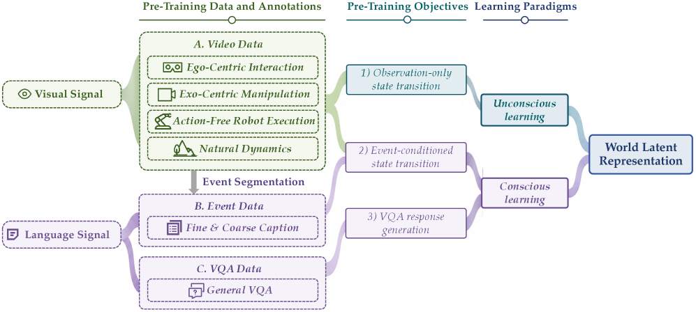
Orca splits pre-training into what it calls unconscious and conscious learning. This corresponds to a distinction between dense, unlabeled dynamics (video) and sparse, language-labeled dynamics (events, VQA).
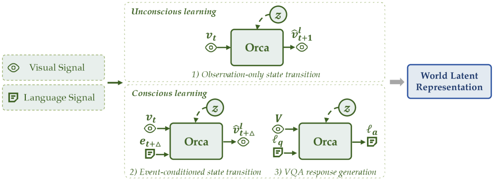
Concretely, the VLM backbone consumes a token sequence of the form <visual token>, <Query 1>, <Instruction>, <Query 2>, where <Query 1> and <Query 2> are learnable query vectors trained from scratch. Three objectives are stacked:
Observation-only state transition (unconscious). Given frame embedding v_t and query q_1, the last-layer hidden state of q_1 is passed through a 2-layer MLP to predict \hat{v}^l_{t+1}. Ground truth v^l_{t+1} comes from a frozen vision encoder. Continuous video supplies dense supervision for motion, occlusion, and object interaction.
Event-conditioned state transition (conscious). Given v_t, q_1, an event description e_{t+\Delta}, and q_2, the last-layer hidden state of q_2 predicts \hat{v}^l_{t+\Delta} through a 2-layer MLP. e_{t+\Delta} can be a task intention, description, or causal premise.
VQA response generation. Standard next-token loss on l_a conditioned on (V, l_q) using the LM head.
Objectives (1) and (2) are supervised in the frozen vision encoder’s latent space rather than in pixel space. This is the key modeling decision: by predicting semantic embeddings instead of pixels, the loss avoids capacity being burned on high-frequency reconstruction and instead concentrates on state-level structure. It is essentially JEPA-style latent prediction with an added language-conditioned branch.
Data and scale
Pre-training uses 125K hours of video and 160M event annotations, plus VQA data. Video supports objective (1); video+events support (2); VQA supports (3).
Scaling behavior
The paper’s central empirical claim is that the combined loss decreases smoothly with data and with model size. At 0.8B and 4B parameters, the total loss (Equation 2 in the paper, summing the three objectives) declines monotonically as video hours scale up, and the 4B curve sits strictly below the 0.8B curve throughout training. No plateau is reported — the authors emphasize that Orca “does not converge quickly” and continues to benefit from more data. This is a weaker claim than a clean scaling law (no exponents are fit in the excerpt provided), but the qualitative shape is what one would want from a foundation-model recipe.
The evaluation protocol for downstream tasks freezes the backbone and trains only the modality-specific decoders (text, image, action). This is the correct test for whether the latent is genuinely general: if the frozen features transfer, the world-latent hypothesis has traction; if not, most of the capability lives in task-specific heads. The excerpt sets up the questions (Q1.1 effectiveness/scaling, Q1.2 latent-quality → downstream) and answers Q1.1 affirmatively, but the specific downstream numbers on the three readouts are not in the sections provided here.
Limitations and open questions
Several concerns are worth flagging. First, latent-space prediction targets are defined by a frozen vision encoder; the ceiling of what Orca can represent is bounded by that encoder’s inductive biases, and any dynamics invisible to it (fine-grained physics, sub-pixel motion) cannot be recovered. Second, the “unconscious/conscious” framing is evocative but the mechanical difference reduces to conditioning on language tokens or not — the biological analogy adds little. Third, the abstract lists modalities beyond vision/language (audio, force, infrared) that this instantiation does not include; the “world” here is video+text. Fourth, the paper’s own summary of downstream results is truncated in the provided sections, so the strength of the frozen-backbone claim remains to be adjudicated against numbers on standard benchmarks (embodied action success rates, image prediction FID/LPIPS, text generation quality). Finally, the bidirectional \Delta<0 objective is stated but its contribution is not ablated in what is shown.
Why this matters
If next-state prediction in a latent space genuinely subsumes next-token, next-frame, and next-action prediction with a shared frozen backbone, it collapses three model families into one and reframes multimodal pre-training around dynamics rather than reconstruction. The scaling curves are the first evidence that this is more than a slogan; whether the frozen latent competes with specialist models on their own turf is the deciding question.
Source: https://arxiv.org/abs/2606.30534
Dockerless: Environment-Free Program Verifier for Coding Agents
Problem
Post-training coding agents on SWE-bench-style tasks depends on a program verifier at two points: filtering SFT trajectories and computing RL rewards. The de facto verifier is execution-based — run the held-out unit tests inside a repository-specific Docker image E_x with pinned dependencies:
r_{\text{env}}(x,y) = \mathbb{1}[\text{tests in } E_x \text{ pass under } y].
Building E_x for every repository is the dominant cost in scaling SWE training data. Many real-world repos lack reproducible environments or usable test suites entirely, so the env-based recipe cannot easily scale beyond curated benchmarks. On the rollout side this is already largely solved — the authors show frontier agents under OpenHands lose only 3.0–13.9 resolve-rate points when the per-repo environment is stripped away. The bottleneck is verification. Existing LLM scorers avoid Docker but grade patches from surface features (diff text, issue text) without inspecting the repo, so they underperform substantially.
Method
Dockerless is an agentic, non-executing verifier r_\phi(x,y)\in[0,1] that judges a candidate patch y against issue x and reference patch y_{\text{ref}} by actively reading the codebase.
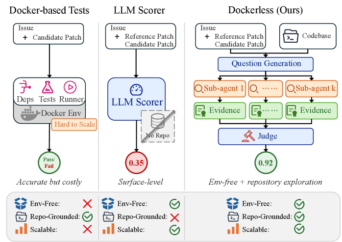
The architecture is a two-stage decomposition:
- Question generation and exploration. Conditioned on (x, y_{\text{ref}}, y), the verifier first proposes K verification questions targeting behaviors that would distinguish a correct patch from a plausible-looking wrong one (e.g., “does the patch handle the empty-input branch that the reference patch modifies in
foo.py?”). Parallel sub-agents each take one question and explore the repo — reading files, tracing callers, inspecting related tests — to return an evidence-backed answer. - Judgment. A final judge conditions on x, y_{\text{ref}}, y, and the K question–answer pairs to emit a correctness verdict.
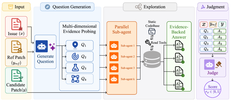
Training uses distillation with rejection sampling against ground-truth env-based labels. A teacher generates full question–answer–judgment trajectories; only trajectories whose predicted verdict matches the ground-truth pass/fail label are retained; the base model is SFT’d on these filtered trajectories.
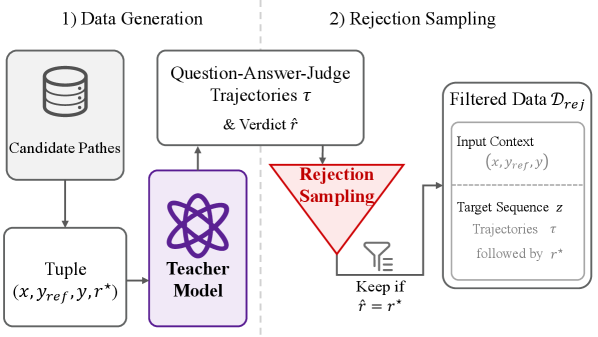
Notably, the verifier itself operates in the env-free regime — sub-agents run in a minimal base image, without needing pinned dependencies or a working test runner. This is what enables the whole post-training pipeline (SFT filtering + RL reward) to be Docker-free.
Results
Verifier quality is measured on a balanced 776-sample trajectory benchmark (500 from SWE-bench Verified, 276 from Multi-SWE-bench Flash). Dockerless beats the strongest open-source verifier by 14.3 AUC points.
Plugged into the full post-training pipeline starting from Qwen3.5-9B, the resulting Dockerless-RL-9B reaches:
- SWE-bench Verified: 62.0% (+2.4 over base)
- SWE-bench Multilingual: 50.0% (+8.7)
- SWE-bench Pro: 35.2% (+2.9)
Compared to the next-best open-source SWE specialist SWE-Lego-8B (41.2 / 19.0 / 16.1), the gains are +20.8, +31.0, +19.1 points. Prior 7B specialists (SWE-Gym-7B, SWE-Dev-7B) are far below, at 11.4 / 3.0 / 3.3 and 10.6 / 4.2 / 4.0.
The controlled comparisons in Table 1 are the interesting part:
- SFT source. Env-SFT-9B (SFT on env-verified rollouts) reaches 60.0 / 48.3 / 33.9; Dockerless-SFT-9B (SFT on Dockerless-verified rollouts) reaches 60.6 / 47.7 / 35.3. Env-free filtering matches env-based filtering.
- RL reward source. With Dockerless-SFT-9B as the starting policy, using DeepSWE-Verifier as reward gives 60.6 / 47.3 / 34.1 — no gain from RL. Using test execution as reward gives 62.4 / 51.3 / 35.7. Using Dockerless as reward gives 62.0 / 50.0 / 35.2 — within 0.4–1.3 points of the execution-based upper bound and substantially better than the alternative env-free reward.
So the end-to-end env-free pipeline recovers essentially all of the benefit that per-repository Docker verification provides, at both SFT and RL stages.
Limitations and open questions
- The verifier is trained by distillation with rejection sampling against ground-truth env-based labels, so bootstrapping the first Dockerless model still requires an env-based labeled corpus. The claim is that env-free scaling applies downstream, not that Docker is ever fully unnecessary.
- Evaluation of the final agent uses env-based scoring on SWE-bench; the verifier’s remaining error modes on non-benchmark repos (where no reference patch y_{\text{ref}} exists) are not directly measured — and the method as described consumes y_{\text{ref}} during verification, which limits applicability to settings with gold patches.
- Test-Execution RL still beats Dockerless RL on all three benchmarks (62.4 / 51.3 / 35.7 vs 62.0 / 50.0 / 35.2). The gap is small but consistent.
- Cost accounting: agentic exploration with K parallel sub-agents per candidate patch is not free; the paper’s framing is that this cost trades favorably against per-repo Docker setup, but concrete verifier compute is not surfaced here.
Why this matters
If verification — not rollout — is the last piece of SWE post-training that structurally requires Docker, removing it opens the door to training coding agents on the long tail of real repositories that have no reproducible environment. Dockerless shows the loss from doing so is under ~1 point of resolve rate versus execution-based rewards, which is likely a worthwhile trade for orders-of-magnitude more training data.
Source: https://arxiv.org/abs/2606.28436
GEAR: Guided End-to-End AutoRegression for Image Synthesis
Problem
Two-stage visual generation — train a VQ tokenizer for reconstruction, freeze it, then fit an autoregressive (AR) transformer over its indices — implicitly assumes the tokenizer’s index distribution is easy to model causally. It isn’t: the tokenizer is optimized only for pixel fidelity and codebook usage, with no signal about which index sequences are learnable under next-token prediction (NTP). Attempts to close the loop via a straight-through estimator (STE) on the \arg\min assignment collapse. GEAR addresses this by co-training tokenizer and AR end-to-end with a stable gradient path, guided by representation alignment (REPA) to DINOv2 features.
Method
The VQ tokenizer is standard: encoder \mathcal{E} maps \mathbf{x}\in\mathbb{R}^{H\times W\times 3} to \mathbf{Z}\in\mathbb{R}^{N\times d}, quantized against codebook \mathcal{C}=\{\mathbf{c}_k\}_{k=1}^K with
q_i = \arg\min_k \lVert \mathbf{z}_i - \mathbf{c}_k \rVert_2^2, \quad \hat{\mathbf{z}}_i = \mathbf{c}_{q_i},
and the composite loss
\mathcal{L}_{\mathrm{VQ}} = \mathcal{L}_{\mathrm{rec}} + 0.1\mathcal{L}_{\mathrm{LPIPS}} + 0.1\mathcal{L}_{\mathrm{GAN}} + 0.05\mathcal{L}_{\mathrm{ent}} + 0.25\mathcal{L}_{\mathrm{commit}}.
The AR has its own embedding table \mathbf{E}\in\mathbb{R}^{K\times d} (not tied to \mathcal{C}), consumes indices q_i and predicts p_\theta(q_i \mid \mathbf{q}_{<i}, c).
The core mechanism is a dual read-out of the codebook assignment (Figure 2c). At each position, GEAR forms both a hard one-hot assignment \mathbf{a}^{\text{hard}}_i \in \{0,1\}^K from the \arg\min and a temperature-scaled soft assignment
\mathbf{a}^{\text{soft}}_i = \mathrm{softmax}\!\left(-\lVert \mathbf{z}_i - \mathbf{c}_k \rVert_2^2 / \tau\right), \quad \tau = 0.1.
The hard branch drives NTP and a “hard” REPA loss that updates only the AR (stop-grad on the tokenizer). The soft branch carries a differentiable REPA loss that bypasses the AR’s upper causal blocks and flows back to update only the tokenizer.
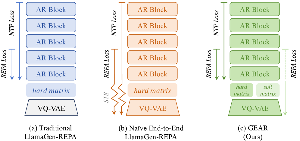
Concretely, gradients from the soft REPA loss can traverse the soft-assignment matrix into \mathcal{E} and \mathcal{C}, but are gated so they never modify AR parameters, and NTP gradients (which are non-differentiable through \arg\min) never try to push through the tokenizer. This is what a naive STE end-to-end does and it collapses. The clean split means the AR steers the tokenizer’s index distribution toward one it can predict, while the tokenizer’s own representation-alignment burden decreases — the tokenizer’s features become less DINOv2-like, while the AR’s internal features become more so, inverting the diffusion-side REPA recipe.
Training happens in two regimes. For ablations, tokenizer and AR are fine-tuned jointly. For main-table comparisons, GEAR runs the joint phase for 400k steps, then freezes the resulting tokenizer and trains a fresh AR on top with the identical budget used by LlamaGen-REPA on the frozen warm-up tokenizer. Any gap between LlamaGen-REPA and GEAR then isolates the tokenizer contribution.
Results
On ImageNet-1K 256×256 class-conditional generation, GEAR’s improved tokenizer transfers into a standard frozen-tokenizer pipeline and matches the AR budget of LlamaGen-REPA. The tokenizer changes are visible in codebook statistics: over the joint fine-tune, top-1 and top-10 cumulative assignment mass increase, usage entropy H drops in nats, and the effective codebook size \exp(H) shrinks — the distribution sharpens onto a smaller set of high-utility codes.
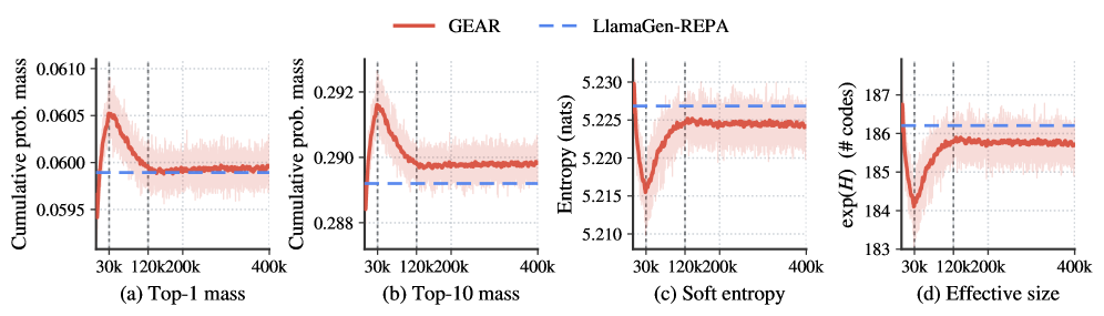
The efficiency payoff is best seen in training dynamics on the 100M-image GPIC corpus, where LlamaGen-REPA and GEAR share encoder, AR architecture, and one-epoch (390k step) budget, differing only in the frozen tokenizer.
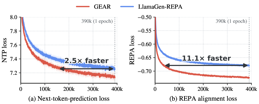
To reach the baseline’s final NTP loss, GEAR is 2.5\times faster; to reach its final REPA alignment loss, 11.1\times faster. The asymmetry is consistent with the mechanism: GEAR has effectively pre-paid part of the alignment cost inside the tokenizer, so the AR spends less capacity aligning to DINOv2 and more on NTP. Evaluation uses gFID/sFID/IS/Precision/Recall over 50k ADM samples for ImageNet, and FD-DINOv2, Precision, Recall, Density, Coverage, MMD on GPIC, plus GenEval, DPG-Bench, and COCO CLIP/FID for text-to-image.
Limitations and open questions
- Full joint training is not run at the largest scales; the reported gains transfer via a frozen post-hoc tokenizer, which sidesteps end-to-end cost but leaves open whether longer joint schedules would compound gains.
- The scheme depends on a DINOv2 alignment target; sensitivity to the choice of representation prior (self-supervised vs. supervised, ViT vs. ConvNet) is not characterized in the excerpts provided.
- Temperature \tau=0.1 governs the softmax read-out; the soft assignment must be sharp enough that the tokenizer’s guidance signal is consistent with the hard indices the AR actually consumes. The stability envelope in \tau, and interactions with the codebook entropy weight (0.05), are not fully mapped.
- The sharpening of codebook usage (Figure 4) reduces effective vocabulary; whether this trades against ceiling reconstruction quality at higher resolutions is unclear.
- The mechanism generalizes in principle to any discrete-index generator (masked, hybrid), but here it is instantiated only for causal AR.
Why this matters
GEAR gives a clean recipe for end-to-end training across a non-differentiable quantization bottleneck by splitting hard and soft assignment paths, and empirically shows that the tokenizer — not just the generator — is where representation-alignment priors should be spent for AR image models. The resulting tokenizer is a drop-in artifact that accelerates downstream AR training by 2.5–11\times on matched budgets, which is the kind of decoupling that makes the technique easy to adopt.
Source: https://arxiv.org/abs/2606.32039
Evolution Fine-Tuning: Learning to Discover Across 371 Optimization Tasks
Problem
LLM-driven evolutionary search (FunSearch, AlphaEvolve, OpenEvolve) has produced state-of-the-art results on open mathematical problems, GPU kernel design, and combinatorial optimization. In these systems the model is a frozen mutation operator; the scaffold owns the search logic — which parent to select, which region to mutate, when to backtrack. Each new task restarts from scratch, and the reasoning built up during a search is discarded when the run ends. The authors ask whether the mutation policy itself — knowing how to evolve a solution — can be pushed into the model weights, and whether such a policy transfers across heterogeneous optimization domains.
Method
Evolution Fine-Tuning (EFT) is supervised mid-training on evolutionary trajectories. The pipeline (Figure 4) is:
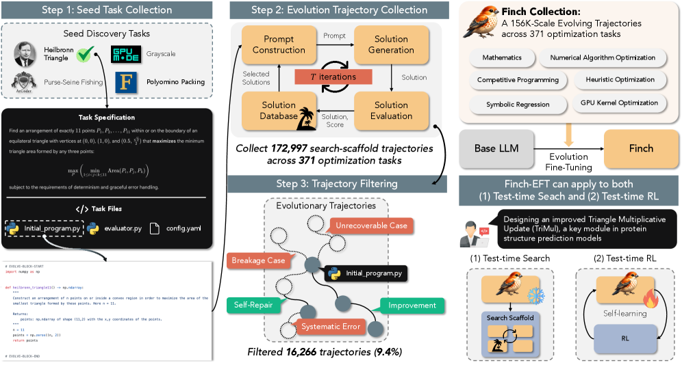
- Collect 371 seed optimization tasks, each with a task specification, an initial candidate solution, an evaluator, and configuration files.
- Run OpenEvolve to produce parent-to-child transitions. Each transition records the prompt, parent code, generated child, evaluator output, score change \Delta s = s(\text{child}) - s(\text{parent}), and execution artifacts.
- Filter unrecoverable trajectories, syntactic breakages, and systematic errors (e.g. timeouts) so that supervision is not dominated by degenerate mutations.
The resulting Finch Collection contains ~156K trajectories across 10 domains. Fine-tuning treats a transition as a conditional generation problem: given the prompt (task spec, parent, feedback), predict the child. Because trajectories are filtered to retain informative transitions — including productive backtracks and successful mutations — the model learns an implicit policy over which edits improve solutions given evaluator feedback. Crucially, EFT is orthogonal to the test-time scaffold: the resulting Finch models can be plugged into OpenEvolve with frozen weights, or further trained with test-time RL.
Results
The authors fine-tune Qwen3/Qwen3.5 at 2B, 4B, 8B, and 9B and compare against the same base model inside OpenEvolve on 22 held-out tasks across five domains (Mathematical Discovery, Algorithm Engineering, System Performance, Competitive Programming, Algorithmic Heuristics). Highlights from Table 3:
- Erdős minimum overlap. Finch-4B reduces the objective from 0.4169 to 0.3865 (+7.31\%); Finch-8B reaches 0.3812, essentially matching the best-known human bound 0.3809 and Claude-Opus-4.6 (0.3819).
- Circle packing n{=}26. Finch-9B improves score from 1.173 (Qwen3.5-9B) to 1.936 (+65.1\%), closing much of the gap to GPT-5/Gemini-3-Pro (2.54) and Claude-Opus-4.6 (2.63).
- Hadamard max-determinant. Finch-8B: 0.502 vs. base 0.452 (+10.9\%); Finch-9B: 0.481 vs. 0.397 (+21.0\%). Not all sizes benefit — Finch-4B regresses to 0.146, suggesting instability at smaller scales on this task.
- ahc058 (algorithm engineering). Base Qwen3.5-9B scores 1.34\times10^8; Finch-9B reaches 5.25\times10^8 (+290\%). Base 2B/4B/8B all score 0, which the authors exclude from the average.
- System performance. On Transaction, Finch-4B jumps from 2732 to 4762 (+74.3\%), exceeding GPT-5 (4237) but below Gemini-3-Pro (4274).
- Aggregate. Average relative gain over the same-size base ranges from +1.56\% (2B) to +10.24\% (9B), monotone in model size.
Notably, several open Finch variants match or exceed proprietary models inside the same scaffold: Finch-8B/9B beat Claude-Opus-4.6 on Erdős, and Finch-4B beats all three proprietaries on Transaction. This is meaningful because the scaffold is held fixed — the delta is entirely attributable to the mutation-operator policy embedded in the weights.
Scaling and transfer
Section 5 reports positive scaling in the number of training tasks: performance on AC2, CP(n{=}26), and PRISM improves monotonically as more of Finch Collection is used. Combined with the size scaling in Table 3, this suggests the collection is not saturating and that gains are not concentrated in tasks similar to training tasks — the evaluation set is largely disjoint from training. The competitive-programming results (CALICO P263 and FrontierCS P301–305) are used as a stress test for cross-domain transfer: Finch appears to compose strategies learned on mathematics and systems tasks when attacking NP-hard contest problems.
Limitations and open questions
- The paper reports isolated regressions (Hadamard at 4B, ahc039 at 2B, EPLB at 9B), and the “Avg. Gain” excludes ahc058 because the base scores zero. The variance across tasks/sizes is not fully characterized.
- Supervision is imitation of OpenEvolve traces produced by whatever LLM populated Finch Collection; the ceiling of EFT is bounded by the teacher distribution unless combined with RL.
- The excerpt does not detail the loss (full-sequence LM loss over the child? weighted by \Delta s?), which matters for reproduction. Filtering criteria beyond breakage/timeout are also under-specified.
- No head-to-head comparison against test-time RL alone, so the marginal value of EFT as a pre-RL initializer is inferred rather than measured.
- Contamination between the 371 training tasks and the 22 evaluation tasks is claimed to be minimized “to the extent possible” but not audited quantitatively.
Why this matters
EFT is a concrete demonstration that the “discovery policy” implicit in evolutionary scaffolds — mutation choice, feedback interpretation, backtracking — can be internalized by open 2–9B models via SFT on filtered search traces, closing the gap to frontier proprietary models inside the same scaffold on tasks like Erdős and circle packing. If the reported task-count scaling holds, this reframes evolutionary search from a per-task test-time procedure into a mid-training data source.
Source: https://arxiv.org/abs/2606.29082
Reinforcement Learning with Metacognitive Feedback Elicits Faithful Uncertainty Expression in LLMs
Problem
LLMs express confidence that is decoupled from their internal (intrinsic) uncertainty: they hallucinate assertively and hedge on things they know. The paper targets faithful calibration (FC), defined as alignment between expressed confidence and intrinsic confidence estimated from response consistency, rather than alignment with ground truth (which is standard calibration). FC is itself a metacognitive task — the model must monitor its own likelihood of being correct — and remains poor even in frontier models (Table 1 reports average cMFG* of 0.70 for Gemini-3.1-Pro, 0.66 for Gemini-3-Flash, 0.61 for GPT-5).
Method
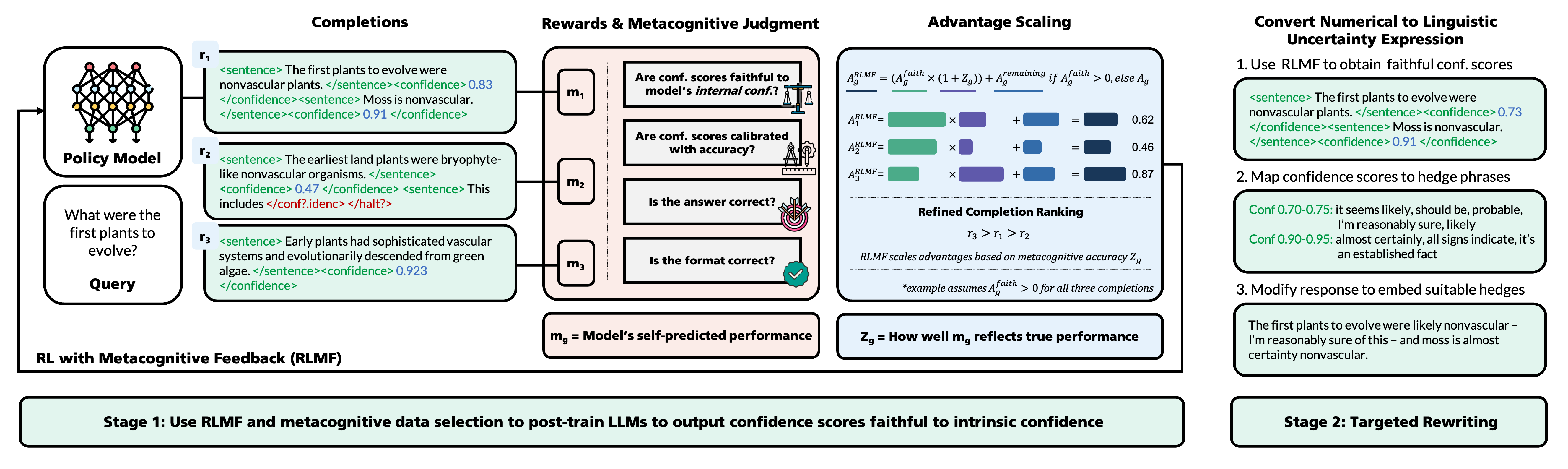
The pipeline is two-stage: (1) RL on numerically expressed sentence-level confidences, then (2) a rewriting stage that maps numerical scores into linguistic hedges. Decoupling avoids re-running RL when user preferences over hedge style change and mitigates GRPO’s mode-collapse tendency on lexical hedges.
RL setup. Given query q, model M_\theta produces G completions, each a sequence of (sentence, confidence) pairs: r_g = \{(s_1,c_1),\ldots,(s_{N_g},c_{N_g})\},\quad g=1,\ldots,G. Intrinsic confidence per sentence is estimated from cross-sample consistency across the G rollouts (dual-use of the GRPO group). Each r_g receives a composite scalar reward \rho_g combining (i) faithfulness of expressed vs. intrinsic confidence, (ii) correctness, (iii) factual calibration (to counter the known factual/faithful tradeoff), and (iv) format adherence.
Following Liu et al., they use unnormalized GRPO advantages: A_g = \rho_g - \bar{\boldsymbol{\rho}}, dropping the \text{std}(\boldsymbol{\rho}) denominator to reduce difficulty bias.

RLMF — metacognitive feedback. The core novelty: rather than accepting \rho_g as the ranking signal, RLMF modulates advantages by the model’s own judgment of completion quality. Concretely, the model is queried for self-judgments over the group, and these judgments reweight the group-relative ranking used in A_g. This turns a monitoring signal (self-assessment) into a regulation signal (policy gradient reweighting), operationalizing the paper’s thesis that models which accurately judge their own performance are better positioned to improve it.
Metacognitive data selection. The same self-judgment mechanism is used to select high-value training instances — examples where model self-assessment discriminates well among candidates — reported to outperform naive active learning selection.
Rewriting stage. After Stage 1 produces faithful numerical scores, a separate rewriting step maps c_i into linguistic uncertainty expressions. This preserves lexical diversity, which the cMFG* metric would not otherwise penalize repetition of.
Results
Main metric is cMFG* (composite metric for faithful generation, higher better), with accuracy (Acc) and Brier score (BS) tracked to check for degradation.
- Llama3.1-8B-Instruct: baseline cMFG* = 0.60 → RLMF 0.84 → RLMF+Rewrite 0.82. Accuracy improves 0.31 → 0.41; BS drops 0.33 → 0.26.
- Qwen3-8B: baseline 0.54 → RLMF 0.83. Accuracy 0.55 → 0.57; BS 0.31 → 0.19.
- Ablation without metacognitive advantage scaling (RL row): Qwen3-8B collapses to 0.51 average (with HE = 0.20, AC = 0.32, SG = 0.38), confirming that plain GRPO on these rewards is unstable and that the metacognitive reweighting is what stabilizes and generalizes learning.
- Vs. baselines: average gains of 29% over prompting (MetaFaith) and 25% over SFT (FUT).
- Vs. proprietary models: 8B RLMF beats GPT-5 by 37%, Gemini-3-Flash by 25%, Gemini-3.1-Pro by 17% on average cMFG*, despite the latter using specialized prompting.
- OOD generalization: trained only on PopQA, RLMF holds up on MATH, SimpleQA, and other tasks unlike FUT, whose gains concentrate on QA formats close to training.
- Training-task robustness (Table 2): switching training data from PopQA to SelfAware yields 0.81 for Llama3.1-8B (vs. 0.84 with PopQA), indicating the method is not sensitive to the specific supervision distribution.
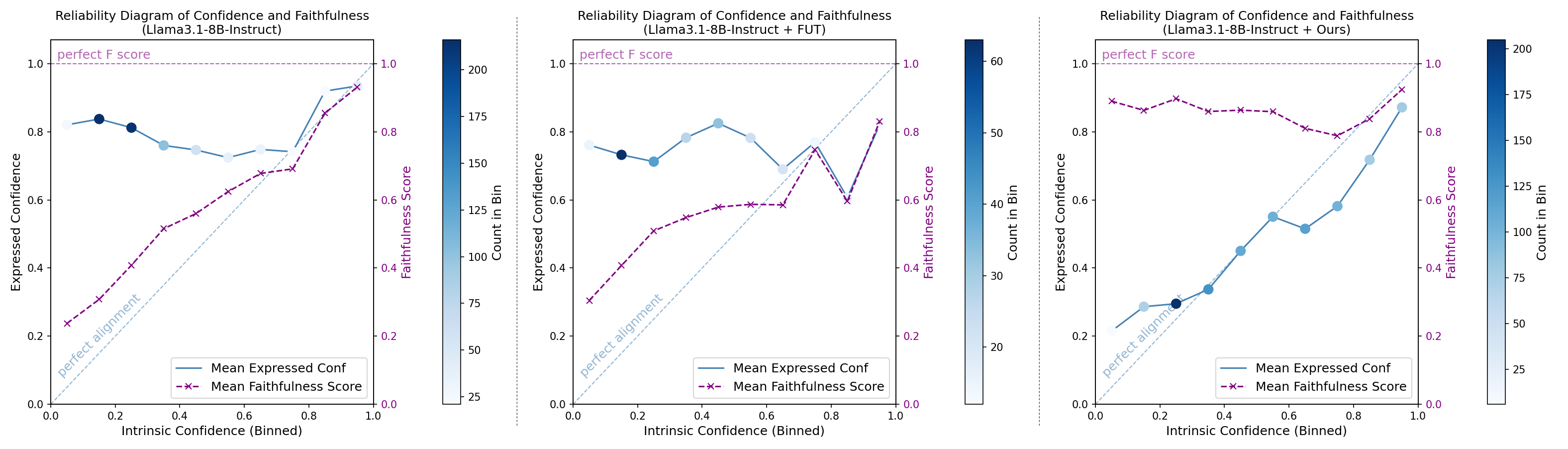
The reliability diagrams show that FUT and base models systematically overshoot at low intrinsic confidence (they cannot express low certainty), while RLMF’s expressed-vs-intrinsic curve tracks the diagonal across the full [0,1] range. This is the clearest evidence that the gains are not just averaging artifacts but reflect faithful monotone behavior at both tails.
Limitations and open questions
- Intrinsic confidence is proxied by response consistency across the GRPO group; this conflates epistemic uncertainty with sampling temperature/format variance. FC is only as meaningful as this proxy.
- Only 8B-class open models are trained; the paper reports no results for training RLMF on frontier-scale models where the metacognitive signal itself may be more reliable and thus give different dynamics.
- The rewriter is trained/prompted separately; its faithfulness under distribution shift (long-form reasoning, code, multi-turn) is not stress-tested here.
- Composite reward weighting is fixed per §C.1.1; the interaction between the metacognitive advantage reweighting and the reward-mixing coefficients is not disentangled.
- The self-judgment used to reweight advantages is itself a model output. When a model’s monitoring is systematically biased, RLMF could reinforce that bias — an open question the reliability diagrams partially, but not fully, address.
Why this matters
Faithful calibration is arguably a prerequisite for downstream trust behaviors (deference, tool use, refusal), and prior methods either helped only in-distribution (FUT) or degraded accuracy (MetaFaith). RLMF shows that a model’s own self-judgment, folded into GRPO advantage estimation, is a strong enough signal to push 8B models past frontier proprietary models on FC without harming accuracy — evidence that metacognition-as-supervision is a tractable RL primitive rather than a philosophical framing.
Source: https://arxiv.org/abs/2606.32032
PolyFlow: Continuous Topology Embedding Flow Matching for Artist-style Mesh Generation
Problem
Artist-quality mesh generation is currently dominated by autoregressive Transformers (MeshGPT, MeshAnything, and successors) that serialize a mesh \mathcal{M} = (\mathcal{V}, \mathcal{F}) into a token sequence \mathbf{s} = (s_1, \dots, s_L) under a fixed z-y-x vertex order and factor p(\mathbf{s}) = \prod_{i} p(s_i \mid s_{<i}). The topology this produces is clean, but decoding is strictly sequential and L grows linearly with face count, making inference orders of magnitude slower than parallel generators. Flow matching and diffusion, which would give parallel decoding, cannot ingest meshes directly: the adjacency structure \mathcal{F} is a discrete combinatorial object that is not closed under Gaussian noise. PolyFlow’s goal is to obtain a continuous state whose Euclidean neighborhood structure encodes discrete adjacency, so that a standard flow-matching Transformer can denoise geometry and topology jointly in parallel.
Method
Continuous topology embedder. The core trick is a pretrained, frozen embedder that maps each vertex v_j (with position and normal) to a continuous vector \mathbf{e}_j \in \mathbb{R}^{d} such that the original discrete edge set can be recovered by thresholding a spacetime distance between embedding pairs. Concretely, an edge (v_j, v_k) \in \mathcal{E} is decoded iff d(\mathbf{e}_j, \mathbf{e}_k) < \tau for some learned/fixed threshold, with the “spacetime” combining Euclidean position and the learned embedding channels. This turns adjacency into a metric-neighborhood predicate on continuous vectors, which is stable under small perturbations — exactly what a diffusion/flow model produces near convergence.
Joint flow state. After pretraining and freezing the embedder, each mesh becomes a per-vertex tensor \mathbf{z} = [\mathrm{xyz},\, \mathrm{normals},\, \mathrm{emb}] \in \mathbb{R}^{B \times V \times D}. All three channel groups are treated as one continuous state; there is no separate discrete branch.
Flow-matching Transformer. A conditional flow-matching objective is used with linear interpolant \mathbf{x}_t = (1-t)\mathbf{x}_0 + t\mathbf{z}, \mathbf{x}_0 \sim \mathcal{N}(0, \mathbf{I}), and target velocity \mathbf{v}^\star = \mathbf{z} - \mathbf{x}_0. The Transformer v_\theta is trained under \mathcal{L} = \mathbb{E}_{t, \mathbf{x}_0, \mathbf{z}, c} \big\lVert v_\theta(\mathbf{x}_t, t, c) - (\mathbf{z} - \mathbf{x}_0) \big\rVert_2^2, with c being point-cloud features from a frozen condition encoder (a point cloud is sampled from the mesh surface at training time).
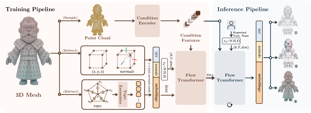
Inference. The user supplies a target vertex count \hat{V}. The model initializes \hat{V} tokens of shape (B, \hat{V}, D) from Gaussian noise and integrates the ODE \frac{d\mathbf{x}_t}{dt} = v_\theta(\mathbf{x}_t, t, c) with an EMA copy of the Transformer over 50 Euler steps. The resulting \mathbf{z} is split channel-wise into positions, normals, and embeddings; edges and faces are then read off by spacetime distance thresholding on the embedding block. Because all vertices are denoised simultaneously, cost is roughly independent of V up to attention scaling, in contrast to the \mathcal{O}(L) decoder passes required by AR baselines. The vertex-count control is exact — a property AR models can only approximate via early stopping.
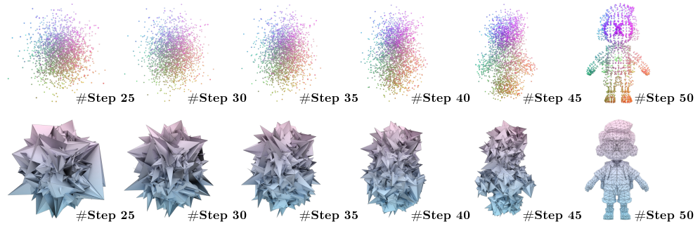
Figure 3 is worth noting mechanically: because adjacency comes from thresholding continuous embeddings, connectivity emerges gradually as embedding clusters tighten. Early steps produce plausible point clouds with noisy faces; late steps snap edges into place without any discrete resampling.
Results
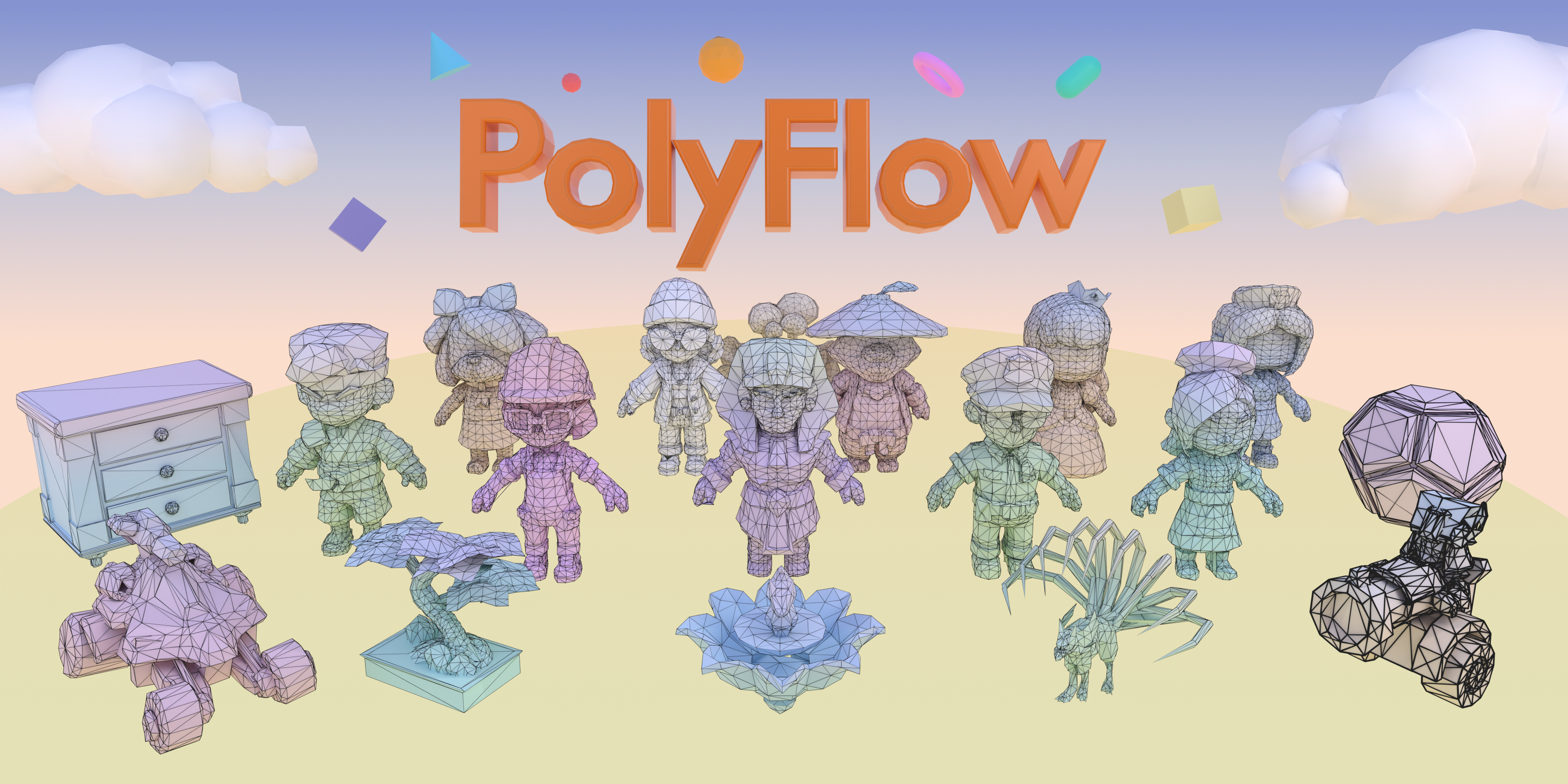
Training uses roughly 5M meshes assembled from public and licensed 3D asset repositories; evaluation is on Toys4K, which is held out. Conditioning is a point cloud uniformly sampled from the target surface. The abstract and pipeline description make two operational claims: (i) fully parallel vertex generation in a single denoising trajectory rather than L AR steps, and (ii) exact vertex-count control at inference, driven by the user-specified \hat{V}. The teaser figure demonstrates artist-style topology (regular quad-like layouts, clean edge loops) at second-scale wall-clock latency — the qualitative regime previously exclusive to AR mesh Transformers.
Limitations and open questions
- The embedder is pretrained and frozen; its capacity bounds the topological complexity the flow can express. Meshes with adjacency patterns poorly covered by the embedder’s training set will not be recoverable regardless of how well the flow denoises.
- Spacetime distance thresholding is a local, pairwise rule. It is unclear how faces (as opposed to edges) are disambiguated when three or more vertices are mutually within \tau — face extraction likely requires additional combinatorial post-processing not detailed in the excerpt.
- The user must specify \hat{V}. This is a feature for controllability but a burden for open-ended generation; there is no obvious mechanism to let the model choose V.
- The provided excerpts do not include quantitative comparisons (Chamfer, normal consistency, topology metrics, latency numbers vs. MeshAnything/EdgeRunner). The efficiency claim relative to AR baselines is architectural rather than empirically substantiated in the sections shown.
- Robustness of thresholding under partial denoising, and whether the ODE step count of 50 can be reduced with higher-order solvers or distillation, are open.
Why this matters
PolyFlow is the first plausible route to combining artist-style mesh topology with parallel, flow-matching-style decoding, by pushing the discreteness of \mathcal{F} into a metric predicate over learned continuous embeddings. If the embedder generalizes, this removes the sequential-decoding bottleneck that has kept high-fidelity mesh generation impractical for interactive tools.
Source: https://arxiv.org/abs/2606.30673
BrainJanus: A Unified Model for Understanding and Generation across Brain, Vision, and Language
Problem
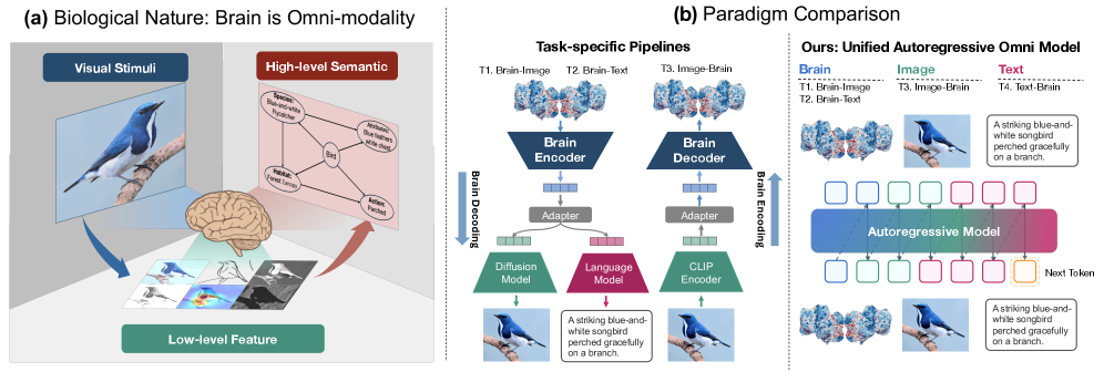
Brain encoding (stimulus \to neural response) and decoding (neural response \to stimulus) have historically been treated as separate pipelines. Decoding work typically bolts an fMRI encoder onto a frozen CLIP/unCLIP/diffusion stack (e.g., MindEye2), while encoding models regress voxel activity from image features. This factorization ignores that cortex integrates visual and linguistic information within a shared representational manifold — a claim supported by semantic tiling results such as Huth et al. (2016). The authors argue that a single model handling all four directions — image\leftrightarrowbrain and text\leftrightarrowbrain — is a more faithful computational analogue and should share statistical strength across tasks.
Method
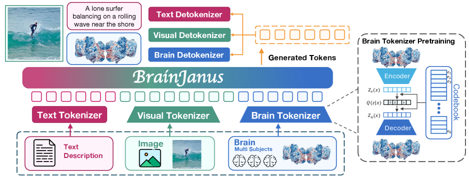
BrainJanus is a two-stage, discrete-token, autoregressive system. Let (x_B, x_V, x_L) \in \mathcal{B} \times \mathcal{V} \times \mathcal{L} denote a tri-tuple of fMRI, image, and caption.
Stage 1 — Unified Brain Tokenizer. Continuous voxel responses x_B \in \mathbb{R}^{N_v} are quantized into a discrete code sequence z_B \in \{1,\dots,K\}^{T_B} living in an “Omni” codebook shared with visual and language tokens. Concretely, the tokenizer produces embeddings e_B = f_\theta(x_B) that are aligned with pretrained visual/text token embeddings before vector quantization, so that a brain token index k has a comparable semantic role to the same index reached from an image or text patch. The alignment objective combines a reconstruction term on x_B and a contrastive/regression term pulling e_B toward the corresponding image and caption embeddings in the Omni space.
Stage 2 — All-in-One autoregressive transformer. Given the tokenizer, any modality reduces to a discrete sequence. Training concatenates task-tagged sequences of the form [\text{task}] \, z_{\text{src}} \, [\text{sep}] \, z_{\text{tgt}} and optimizes the standard next-token loss
\mathcal{L} = -\sum_{t} \log p_\phi(z_t \mid z_{<t}).
Four tasks are mixed during SFT: image\tobrain, text\tobrain, brain\toimage, brain\totext. Because the tokenizer, vocabulary, and objective are shared, inference for any direction is just conditional generation from the same backbone — no diffusion prior, no unCLIP head.
Data and captions. Experiments use the Natural Scenes Dataset (NSD), following the MindEye2 protocol on Subjects 1, 2, 5, 7 with 9,000 unique training images and a shared 1,000-image test set (3 trials each). Because original COCO captions are terse, the authors re-caption the 73k NSD image pool with Qwen3-VL-235B-A22B-Instruct, and show the synthesized captions have higher image-caption semantic similarity than the COCO originals.
Results
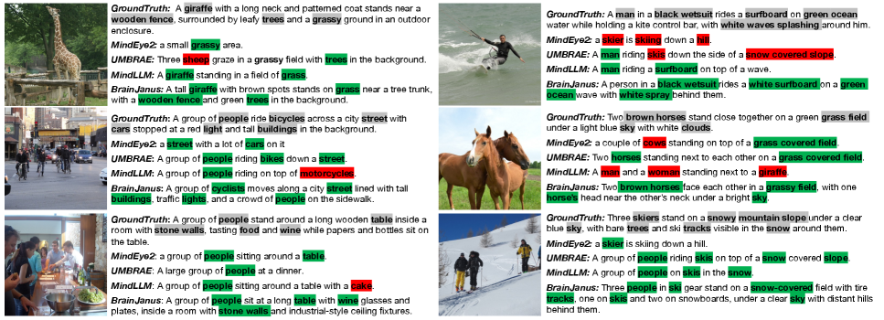
Brain-to-image reconstruction (Table 3, NSD test set). BrainJanus is the only fully autoregressive brain-to-image system compared. Against diffusion-based SOTA (MindEye2, UMBRAE, Ozcelik and VanRullen, Takagi and Nishimoto), it reports PixCorr 0.173, SSIM 0.292, AlexNet(2) 90.3%, AlexNet(5) 97.1%, Inception 94.7%, CLIP 94.4%, EfficientNet 0.656, SwAV 0.372. MindEye2 remains ahead on low-level pixel metrics (PixCorr 0.322, SSIM 0.431), but BrainJanus is competitive to superior on high-level semantic metrics — AlexNet(5) 97.1% vs. 98.6%, Inception 94.7% vs. 95.4%, CLIP 94.4% vs. 93.0%. Notably, BrainJanus beats a Qwen3-VL-235B “caption\toimage” oracle on AlexNet(2/5) (90.3/97.1 vs. 85.0/94.2), suggesting the decoded latent carries information beyond what a caption reconstructs.
Zero-shot brain-to-image. Training on brain-to-text pairs only and then generating images at inference yields PixCorr 0.077, SSIM 0.257, AlexNet(2) 69.3%, CLIP 77.3%. Weaker than supervised, but well above chance and above several early diffusion baselines on semantic metrics — evidence that the shared Omni space transfers direction implicitly.
Brain-to-text. Qualitative comparisons against MindEye2, UMBRAE, and MindLLM show fewer object-identity errors and better preservation of action attributes. Detailed numerical language metrics are not shown in the excerpt but the figure highlights consistent semantic-match gains.
Limitations and open questions
- Low-level fidelity lags MindEye2 (PixCorr 0.173 vs. 0.322). Discrete tokenization at moderate codebook resolution loses fine spatial detail that pixel-level diffusion decoders retain.
- Only 4 NSD subjects are evaluated; cross-subject generalization of the tokenizer, and whether the Omni space is subject-invariant, is not quantified in the shown tables.
- The tokenizer training relies on paired (x_B, x_V, x_L) triplets; scaling to modalities where paired data is scarce (EEG with text, MEG, etc.) is untested despite the “brain signals” framing.
- Encoding results (image\tobrain, text\tobrain) are not covered in the excerpt shown, so it is unclear whether joint training helps or hurts the forward direction relative to specialized encoders.
- Reliance on synthetic captions from Qwen3-VL introduces a distribution shift; the reported CLIP/Inception gains partly reflect that the model was trained to match richer captions than the COCO ground truth.
Why this matters
Recasting brain encoding and decoding as next-token prediction in a shared discrete space collapses a fragmented stack (CLIP + unCLIP + diffusion prior + captioner) into one autoregressive model with competitive semantic performance and native any-to-any inference, including a nontrivial zero-shot brain-to-image transfer. If the Omni-space alignment holds up across subjects and modalities, it provides a cleaner substrate for studying multimodal cortical representation than task-specific pipelines.
Source: https://arxiv.org/abs/2606.30319
Hacker News Signals
Claude Code is steganographically marking requests
Anthropic’s Claude Code CLI embeds hidden metadata into prompts sent to the API — a form of steganographic watermarking at the application layer. The discovery, documented at thereallo.dev, shows that the tool injects invisible Unicode characters (specifically zero-width or variation-selector codepoints) into system prompts or user-turn text before the request hits the network. These characters encode structured information about the request origin, likely tooling version, session context, or operator identity.
The practical consequence is that Anthropic can distinguish Claude Code-originated traffic from raw API calls without relying solely on HTTP headers or API key metadata, both of which can be trivially spoofed or stripped. This matters for rate-limiting, abuse detection, and potentially for behavioral tuning — the model or the serving infrastructure could alter responses based on detected provenance.
From a security standpoint, the technique is a form of out-of-band signaling hidden in-band. The watermark survives copy-paste of the prompt text, which is the point: it is more robust than a header. However, it is trivially detectable once you know to look for non-printing Unicode in the UTF-8 byte stream, and equally trivially stripped with a Unicode normalizer or a whitelist filter on codepoints.
The broader concern raised in the thread is consent and transparency: users of Claude Code are not informed that their prompts carry embedded provenance markers. This touches on supply-chain trust — if you relay Claude Code output into another system’s prompt, you are unknowingly forwarding Anthropic’s metadata. There are also implications for any downstream system that fingerprints or audits prompts, since the invisible characters change content hashes.
Technically, this is not novel — steganographic Unicode abuse has been documented in prompt injection research and in exfiltration PoCs — but its deployment in a first-party production CLI is notable.
Source: https://thereallo.dev/blog/claude-code-prompt-steganography
From brain waves to words: a new path to communication without surgery
Meta’s Brain2Qwerty project decodes imagined or attempted typing keystrokes from non-invasive EEG and MEG recordings. The system targets locked-in or severely motor-impaired users and works without implants. The core pipeline processes high-density sensor data through a neural sequence model that maps temporal brain-signal patterns to character-level outputs on a QWERTY layout, exploiting the fact that imagined finger movements for specific keys produce distinguishable cortical signatures.
MEG (magnetoencephalography) provides higher spatial and temporal resolution than EEG, though it requires large, expensive superconducting hardware. The model architecture is a convolutional front-end for spatial filtering of the sensor array, feeding into a temporal sequence model (transformer-based, per the paper backing the blog post), trained to predict key identity from windows of neural activity. A language model rescoring stage applies prior probability over plausible character sequences to reduce the raw decoding error rate.
Reported accuracy reaches around 80% character-level correctness under MEG with the LM rescorer, degrading significantly under EEG alone. Throughput is low — on the order of a few characters per second — making this viable for communication but not yet for general-purpose text input.
Key limitations: MEG is not wearable or deployable outside specialized labs. EEG accuracy is substantially worse. The system requires per-subject calibration with significant training data collection. Generalization across sessions and days remains an open problem due to signal non-stationarity. The “without surgery” framing is accurate but can mislead — MEG is not a bedside or home device. The interesting technical question is whether the approach transfers to dry-electrode portable EEG systems, which would be the actual path to deployment.
Source: https://ai.meta.com/blog/brain2qwerty-brain-ai-human-communication/
Zluda 6 release (run unmodified CUDA applications on non-Nvidia GPUs)
ZLUDA is a drop-in CUDA compatibility layer that lets unmodified CUDA binaries run on AMD (and historically Intel) GPUs. Version 6 continues the project’s post-AMD-sponsorship-cancellation independent trajectory. The mechanism is a reimplementation of the CUDA runtime and driver APIs (libcuda.so / nvcuda.dll shims) that translates CUDA calls to ROCm/HIP at runtime. PTX (Parallel Thread Execution) and SASS are handled via an IR translation layer that converts NVIDIA’s virtual ISA to AMD’s RDNA/CDNA ISA through LLVM.
The update-q1q2-2026 post details several improvements: better PTX coverage including previously unsupported atomic operations and warp-level primitives, improved performance on memory-intensive kernels through better buffer aliasing in the translation layer, and fixes to the CUDA stream and event synchronization model which previously caused race conditions on AMD hardware due to different memory consistency semantics.
Correctness is the hard problem here. CUDA’s memory model and AMD’s memory model are not identical, particularly around the strength of atomics and the behavior of __threadfence. ZLUDA has to emulate NVIDIA semantics using stronger (more expensive) AMD fences in some cases. For applications that underspecify their synchronization — which is common in practice — this produces correct results at the cost of performance.
The practical target audience is users who need to run pre-built CUDA binaries (PyTorch, compiled ML kernels, commercial software) on AMD hardware without access to source. For open-source code, recompiling with HIP or ROCm is generally preferable. ZLUDA does not promise performance parity; the translation overhead is real, and driver-level optimizations Nvidia applies for specific CUDA patterns are not replicated.
Source: https://vosen.github.io/ZLUDA/blog/zluda-update-q1q2-2026/
I ported Kubernetes to the browser
This ngrok engineering post describes running a functional Kubernetes control plane inside a browser tab using WebAssembly. The approach compiles the relevant Go-based Kubernetes components (kube-apiserver, etcd, controller-manager, scheduler) to WASM targets, runs them in a Web Worker to avoid blocking the main thread, and uses an in-memory network stack to connect the components without actual sockets.
The non-trivial parts are: (1) etcd depends on bbolt which does file I/O — this is shim-replaced with an in-memory store; (2) the Go runtime’s goroutine scheduler and timer mechanisms work under WASM but with higher overhead than native; (3) kubelets and actual pod scheduling cannot run in-browser because there is no container runtime, so the demo is purely control-plane and does not schedule real workloads.
The use case described is interactive Kubernetes API documentation and tutorial tooling — users can kubectl apply against a real API server running locally in their browser without any server-side infrastructure. This is technically legitimate: the WASM control plane responds with accurate API semantics, validates manifests against real schema, and returns real watch/list responses.
The engineering challenges in getting large Go programs to compile to WASM are non-trivial: build tags, CGO dependencies, file system access patterns, and network syscalls all require stubs. The post is reasonably detailed on which shims were needed. Memory usage is substantial — running etcd + apiserver in a browser tab consumes several hundred MB. Performance is acceptable for interactive use but not benchmarked under load.
This is a clean example of using WASM as a sandboxed embedded runtime rather than a performance optimization path.
Source: https://ngrok.com/blog/i-ported-kubernetes-to-the-browser
We found a bug in the hyper HTTP library
Cloudflare’s post documents a correctness bug in the hyper Rust HTTP library related to HTTP/1.1 request pipelining and connection reuse. The bug manifests when a client sends pipelined requests on a keep-alive connection and the server closes the connection mid-pipeline: hyper would, under specific timing conditions, attribute a response to the wrong request in the pipeline, causing response body data to be delivered to the incorrect caller.
The root cause is in hyper’s internal state machine for tracking in-flight pipelined requests. A response received after a connection-close signal could be incorrectly matched to a pending request slot if the slot recycling logic ran before the pipeline flush completed. This is a logical race, not a data race — hyper is otherwise memory-safe — but the outcome is that a caller receives another caller’s response body bytes, which is a serious confidentiality issue in a multiplexed context (e.g., a reverse proxy serving multiple tenants).
Cloudflare’s detection path is interesting: they noticed response body length mismatches in their proxy layer’s own accounting, which triggered an anomaly in their internal consistency checks. Pure unit tests would not reliably catch this because it depends on the interleaving of async task polls in Tokio’s executor.
The fix involves tightening the ordering guarantees in the pipeline state machine so that response-to-request matching is validated after the connection state is stable. The post is a good example of the class of bugs that Rust’s ownership model does not prevent: logical protocol state machine errors are not memory safety violations.
Source: https://blog.cloudflare.com/hyper-bug/
Zig SPIR-V Backend Progress
The Zig compiler’s SPIR-V code generation backend — targeting GPU compute via Vulkan/OpenCL — has reached a level of completeness sufficient to compile non-trivial Zig programs for GPU execution. The devlog entry covers recent progress: improved handling of Zig’s comptime evaluation in the SPIR-V context, struct layout correctness under SPIR-V’s strict alignment rules, and support for more of Zig’s control flow constructs including defer and error unions.
SPIR-V is a typed SSA IR with explicit entry points, execution models, and capability declarations. Mapping Zig’s semantics to it is harder than mapping to LLVM IR because SPIR-V is more constrained: no recursion, limited pointer arithmetic, explicit address spaces (Function, Private, Workgroup, StorageBuffer), and no dynamic dispatch. Zig’s comptime system helps here — much of what would require runtime generics in other languages resolves at compile time and produces monomorphized SPIR-V that fits the model cleanly.
The current gaps noted are: no support for Zig’s allocator interface in GPU code (expected, since dynamic allocation is not available in SPIR-V), limited debug info emission, and incomplete coverage of Zig’s standard library for the SPIR-V target. The backend targets zig build -target spirv64-vulkan style invocations and is intended to replace or complement the existing path through spirv-cross for shader code.
For the systems/GPU programming community this is significant: Zig’s explicit memory management, no hidden control flow, and comptime metaprogramming make it a technically well-suited language for GPU kernels if the backend reaches production quality.
Source: https://ziglang.org/devlog/2026/#2026-06-26
Reading the internals of Postgres: Database cluster, databases, and tables
This walkthrough covers the physical layout of a PostgreSQL database cluster on disk, which is directly relevant to anyone debugging storage issues, writing extensions, or understanding Postgres performance at the page level. A Postgres cluster is a single $PGDATA directory managed by one postmaster process; it contains multiple databases, each mapped to a subdirectory named by its OID under $PGDATA/base/.
Each table is stored as one or more 8 KB page files (segments capped at 1 GB by default). The heap file format has a fixed page header (PageHeaderData) containing LSN for WAL, checksums, free space pointers, and the line pointer array. Tuples are stored from the end of the page growing toward the header; the line pointer array (item identifiers) grows from the header forward. This bidirectional growth means free space is in the middle of the page, inspectable via pg_freespace.
Each tuple has its own header (HeapTupleHeaderData) carrying xmin/xmax transaction IDs for MVCC visibility, ctid (physical location for forwarding after updates), null bitmap, and OID if the table has one. The MVCC model means a row update does not overwrite in place — it writes a new tuple version and marks the old one with xmax. Vacuuming reclaims dead tuple space by scanning for tuples where xmax is committed and no active transaction can see the old version.
The post also covers the pg_class, pg_attribute, and pg_namespace catalog tables that map OIDs to human-readable names, which is the correct entry point for understanding how \d tablename in psql translates to physical storage.
Source: https://www.buraksen.dev/articles/internals-of-postgresql-db-cluster-and-tables
6 years and 360 patches to clean all instances of strncpy out of the Linux kernel
strncpy has a design that is hazardous in virtually all real uses: it pads the destination with null bytes up to the specified length but does not guarantee null-termination if the source is longer than the destination. This means code that assumes strncpy(dst, src, n) produces a null-terminated string is wrong whenever strlen(src) >= n, which is exactly the condition where buffer safety matters most.
The Linux kernel had accumulated hundreds of strncpy call sites over decades. The replacement campaign, completed over approximately six years and ~360 patches, substituted strscpy (introduced in kernel 4.3), which always null-terminates, returns the length written or -E2BIG on truncation, and does not null-pad. This makes truncation detection tractable — callers can check the return value rather than having silent data corruption.
The difficulty was not mechanical substitution but auditing each call site: some uses deliberately relied on the null-padding behavior (for fixed-size protocol fields that must be zero-padded, strncpy is correct); others used the return value incorrectly; others had subtle length arithmetic errors that strscpy’s different semantics would expose. Each patch required understanding the invariants of the surrounding code.
This is a case study in the long tail of C safety remediation. The compiler cannot warn on strncpy in the general case because the hazard is semantic, not syntactic. GCC and Clang added -Wstringop-truncation which catches some patterns but not all. The kernel’s solution was social and procedural as much as technical: a sustained multi-year review effort rather than a single automated transformation.
Source: https://smist08.wordpress.com/2026/06/25/linux-kills-strncpy/
Noteworthy New Repositories
myccarl/ai-shortVideo-pipeline
An end-to-end pipeline for automated short-video production, designed around a microservices architecture with a FastAPI orchestration layer and Spring Boot API gateway. The system integrates multiple generative models (image, video, TTS, music) behind a multi-model failover strategy with circuit breakers, so degraded provider endpoints do not halt production. Metering and distributed tracing are first-class — the observability stack covers per-request latency, token costs, and model-specific error rates.
The AI quality gating is the most technically interesting layer. Prompt anchoring ties downstream model calls to a canonical semantic template, reducing subject drift across cuts. CLIP consistency scoring measures frame-to-frame and audio-cover semantic alignment before accepting a segment. AV sync auto-rescue detects drift between generated audio and video timestamps and attempts re-alignment without re-generating the full clip.
This is a reasonable starting point for anyone building a production video automation service who wants quality checks beyond simple rule-based filters. The circuit-breaker and failover logic is directly reusable for any multi-provider LLM or generative-media backend.
Source: https://github.com/myccarl/ai-shortVideo-pipeline
NotASithLord/peerd
Peerd runs an AI agent loop as a browser extension (Chrome and Firefox), eliminating the conventional backend server from the architecture. The agent can directly drive browser tabs — reading DOM state, clicking, filling forms — using the WebExtensions API as its action space. Sandboxed compute is available client-side: JavaScript notebooks and WASM-compiled Linux VMs (likely via v86 or a similar emulator), enabling the agent to execute code without any outbound compute calls.
Output artifacts are shared peer-to-peer rather than through a central server, presumably via WebRTC data channels or a similar browser-native transport. BYOK (bring your own key) means model inference calls go directly from the browser to the provider endpoint; there is no telemetry or proxying layer.
The security model is worth scrutinizing: browser-native agent execution collapses the isolation boundary between the agent and the user’s authenticated sessions. However, for local-only or low-trust-surface use cases this trade-off buys significant simplicity. The architecture removes the operational overhead of running a persistent backend and is fully air-gap compatible once the extension and WASM images are loaded.
Source: https://github.com/NotASithLord/peerd
cobusgreyling/loop-engineering
Loop engineering is a design discipline focused on structuring the human-agent-tool interaction cycle — specifically, how prompts, context windows, tool calls, and review steps should be composed when AI coding agents are doing substantial work. This repository collects practical patterns, starter templates, and three CLI tools targeting that workflow.
loop-init scaffolds a project with agent-aware structure (likely including system-prompt files, tool manifests, and context budgeting configurations). loop-audit analyzes an existing agent loop for common failure modes such as unbounded context growth, missing review gates, or ambiguous tool descriptions. loop-cost estimates token and monetary cost for a given loop configuration before execution.
The conceptual framing is credited to Addy Osmani and Boris Cherny’s work on AI-assisted development workflows. What distinguishes this from generic LLM prompt libraries is the explicit focus on the iterative loop structure — prompt, execute, observe, re-prompt — rather than one-shot generation. With 4600+ stars it has traction as a reference for teams formalizing how they integrate coding agents into CI and development pipelines.
Source: https://github.com/cobusgreyling/loop-engineering
DSB-117/brainblast
Brainblast targets a specific and underserved failure mode in AI-assisted software development: silent integration traps that compile and deploy cleanly but are semantically wrong. The canonical examples are zero-revenue billing configurations (e.g., a payment integration that never charges), auth bypasses that look like valid code, and irreversible architectural choices baked in at generation time.
The tool combines a research/analysis phase that predicts which traps a given AI agent is likely to introduce — presumably via static analysis, pattern matching against known agent failure modes, or LLM-assisted review — with a CI enforcement phase that embeds checks ensuring those specific traps stay fixed once caught. The npx brainblast CLI makes it drop-in for Node-based projects.
The value proposition is shifting quality gates left of production: rather than catching a misconfigured Stripe webhook in a postmortem, the trap is identified at agent-generation time and pinned. The CI integration means regression is caught automatically. This is most useful in organizations where agents are writing non-trivial business logic with external service integrations.
Source: https://github.com/DSB-117/brainblast
eli-labz/Third-Eye
Third-Eye is a production-grade OSINT (open-source intelligence) aggregation platform providing situational awareness across multiple intelligence domains simultaneously. The “multi-domain” framing suggests it ingests and correlates data across network intelligence (IP reputation, BGP, certificate transparency), social/web intelligence, geospatial signals, and possibly dark-web or paste-site monitoring.
Production-grade here implies it is designed for continuous operation rather than ad-hoc querying: persistent data stores, scheduled collection jobs, and normalized cross-domain entity resolution so that an IP address, domain, and social handle can be linked into a unified threat or entity graph. With nearly 900 stars it has attracted significant attention from the security and threat-intelligence communities.
Practically, this fills the gap between single-purpose OSINT tools (Shodan queries, whois lookups) and expensive commercial platforms. For a red team, SOC analyst, or researcher who needs to correlate signals across domains without stitching together five separate API wrappers, a unified platform with a shared data model has real operational value.
Source: https://github.com/eli-labz/Third-Eye
datalab-to/lift
Lift is a document structured-data extraction library from the team behind Datalab. It targets the common problem of pulling typed, schema-conformant records out of heterogeneous document formats — PDFs, scanned images, HTML, and similar — where layout and formatting are part of the information structure rather than incidental.
The architecture almost certainly wraps a vision-language model or document-understanding model (possibly Marker or a similar pipeline also from Datalab) with a structured output layer enforcing JSON Schema or Pydantic-style type constraints. The emphasis on speed and accuracy together suggests the extraction backend is optimized for batched inference rather than pure API passthrough.
The practical differentiator versus a raw GPT-4o call with a JSON schema is pipeline-level reliability: consistent field extraction across document layout variations, handling of multi-page tables, and validation that the extracted structure is well-formed before returning. At 687 stars it is gaining adoption likely because it sits at the right abstraction level — above raw OCR, below a full document-processing platform — for developers building data ingestion pipelines.
Source: https://github.com/datalab-to/lift
dongshuyan/compass-skills
COMPASS (司南) is a personal alignment skills operating system for AI agents — a framework for defining, composing, and routing task-specific behavioral modules (“skills”) such that an agent’s responses and actions can be personalized and controlled at a fine-grained level. The “personal alignment” framing distinguishes it from generic agent frameworks: the goal is adapting agent behavior to individual user preferences, work styles, and task contexts rather than optimizing for a single global objective.
Technically, a “skills OS” in this context likely means a registry of parameterized prompt modules or tool-call patterns, a routing layer that selects and composes skills based on task classification, and a persistence layer that stores user-specific calibration. The total-control (总控) designation suggests a meta-agent or orchestrator sits above individual skill modules and manages execution order, context injection, and conflict resolution between skills.
With 506 stars and bilingual documentation (Chinese and English), it is positioned as both a research artifact and a practical starting point for building personalized agent systems, particularly relevant for productivity and knowledge-work applications.
Source: https://github.com/dongshuyan/compass-skills
Nigh/show-me-the-story
A self-hosted long-form fiction generator distributed as a single Go binary with an embedded web UI. The architecture is deliberately minimal: no database dependency, no cloud services, just a binary that speaks to any OpenAI-compatible API endpoint (local or remote). This makes it compatible with Ollama, LM Studio, or any self-hosted inference backend.
The generation pipeline is multi-stage and editorially structured: the model first produces a hierarchical outline, then writes chapter by chapter, with each chapter passing through review, foreshadowing consistency check, and fact-check steps before being accepted. A final full-book polish pass runs after all chapters are complete. This staged approach addresses a well-known failure mode of LLM long-form generation — incoherence and contradiction accumulation across tens of thousands of tokens — by maintaining structured intermediate representations rather than generating the full text in one pass.
Bilingual support (Chinese and English) is built in. The Go single-binary distribution means deployment is a single file copy, with no runtime dependencies. For researchers studying LLM narrative coherence or developers building writing tools, it provides a clean reference implementation of outline-grounded iterative generation.