Daily AI Digest — 2026-06-23
arXiv Highlights
CLI-Universe: Towards Verifiable Task Synthesis Engine for Terminal Agents
Problem
Training data for terminal agents — LLMs that operate a shell to accomplish multi-step engineering tasks — is the binding constraint on progress. Existing synthesis pipelines (e.g., SkillSynth, Nemotron-Terminal, TerminalTraj) tend to start from surface artifacts (a repo, a man page, a snippet) and retrofit a task around them. The resulting instructions are often underspecified, the execution paths shallow (a few commands), and the verification tests brittle: tests pass on trivially incorrect solutions or fail on correct ones, yielding weak or actively misleading SFT/RL signal. CLI-Universe targets this gap with a synthesis engine designed to produce tasks that are (i) semantically grounded in real technical material, (ii) instantiated as Dockerized executable environments, and (iii) guarded by tests that have been screened for fail-to-pass discriminability.
Method
The pipeline has three stages (Figure 1).
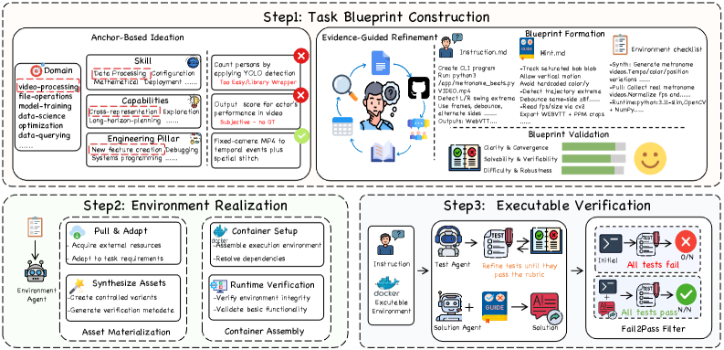
Stage 1 — Blueprint construction. Candidates are sampled as tuples across four axes: domain (e.g., systems, data, devops), skill type, capability, and engineering pillar. Each tuple seeds a research agent that performs iterative deep research over real-world technical sources (docs, issues, tutorials), accumulating evidence which it folds back into a structured task specification. The output is a blueprint: instruction, required assets, expected end-state, and rubric items. The taxonomy-then-ground design is the key contrast with retrofit pipelines — task semantics are decided before any artifact is bound, so the artifact must be found or built to satisfy the spec rather than the spec being warped to fit a found artifact.
Stage 2 — Environment realization. Each blueprint is compiled into a Docker container with materialized assets (filesystem layout, services, network configuration, seeded state). A runtime check confirms the environment boots and the declared preconditions hold.
Stage 3 — Validation with executable filtering. Two independent agents operate on the realized environment:
- A test agent synthesizes rubric-gated tests from the blueprint’s checklist. Tests are gated against the rubric to prevent the common failure mode where a test asserts on an incidental artifact rather than the rubric item.
- A solution agent produces a reference trajectory.
Filtering applies (a) hint-conditional filtering — discarding tasks the solution agent can only complete given over-specified hints (a proxy for trivial tasks) — and (b) strict fail-to-pass checking: the empty/no-op state must fail the tests, and the reference solution must pass. Only candidates surviving all gates are retained.
Across the full funnel only 33.6% of candidates make it through; the remaining roughly two-thirds are killed by environment-build failure, rubric-test mismatch, or fail-to-pass violations.
Results
Models are Qwen3-dense at 8B/14B/32B, SFT’d on 6k trajectories distilled from Kimi-K2 on CLI-Universe tasks. Evaluation uses the Terminus 2 scaffold (200 turns/task, avg@4) on Terminal-Bench 1.0 and 2.0, plus BFCL v4 and VitaBench for generalization.
On TB 2.0, CLI-Universe-32B reaches 33.4, against open-data 32B baselines:
- SkillSynth-32B: 29.6
- Nemotron-Terminal-32B: 27.4
- TerminalTraj-32B: 22.0
The 32B model also exceeds substantially larger open-weight systems — Qwen3-Coder-480B at 23.9 and Kimi-K2-Instruct-1T at 27.8 — suggesting data quality dominates parameter count in this regime. A gap to Claude-Opus-4.5 (57.8) remains. The advantage is preserved at 8B and 14B, indicating the training signal is not specific to a single scale.
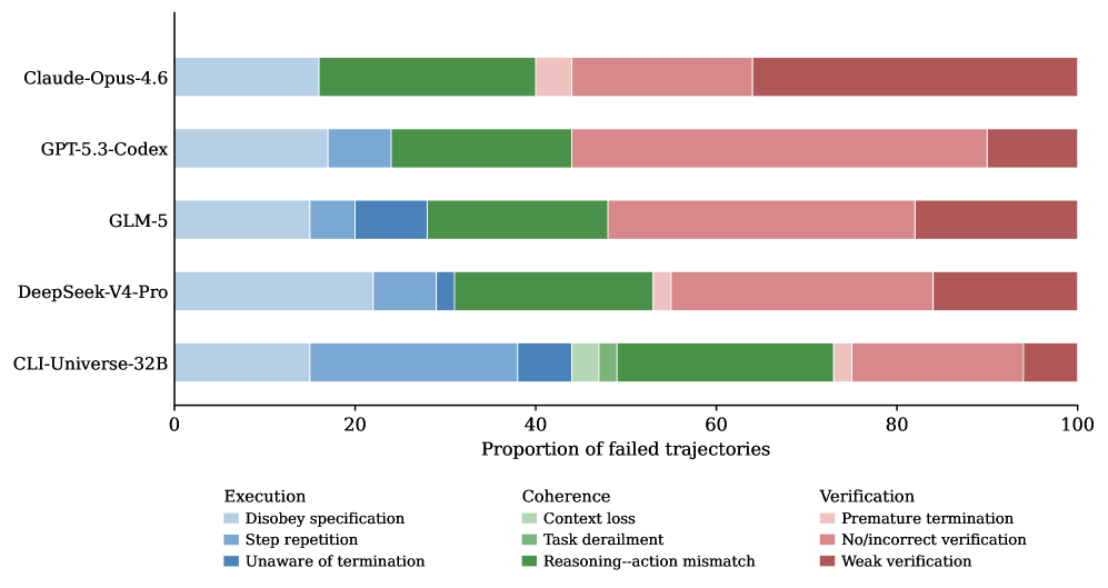
A failure-mode attribution on remaining TB 2.0 failures (Figure 5) breaks errors into nine mutually exclusive causes across Execution (spec disobedience, step repetition, missed termination), Coherence (context loss, derailment, reasoning–action mismatch), and Verification classes. This is useful because it isolates what the data still fails to teach: training on CLI-Universe shifts mass off Verification/Coherence errors but execution-level failures (notably step repetition and missed termination) remain prominent — these are arguably scaffold and decoding issues as much as data issues.
Limitations and open questions
- Distillation dependence. Trajectories come from Kimi-K2; the 32B student’s ceiling is shaped by the teacher’s behaviors, and the work does not disentangle data-quality from teacher-quality contributions.
- SFT only. No RL is reported on top of CLI-Universe data, despite the verifier infrastructure being exactly what an RL loop would need. Whether the rubric-gated tests provide a stable reward remains untested.
- 33.6% yield implies the engine is expensive; cost-per-retained-task is not reported, nor is whether failure modes during synthesis correlate with task difficulty (i.e., is the engine systematically discarding the hardest tasks?).
- No ablation isolating the contribution of taxonomy-seeded sampling vs. evidence-guided research vs. fail-to-pass filtering. Given the pipeline’s complexity, identifying which gate carries the signal would inform reproduction.
- Generalization claims for BFCL v4 and VitaBench are referenced but not quantified in the excerpts here.
Why this matters
Terminal agent benchmarks are saturating with closed models while open systems stall on data quality. CLI-Universe argues, with credible numbers, that a verifier-first synthesis pipeline lets a 32B model match or beat open systems an order of magnitude larger — reframing the open-vs-closed gap as a data-engineering problem rather than a scale problem.
Source: https://arxiv.org/abs/2606.22883
BioMatrix: Towards a Comprehensive Biological Foundation Model Spanning the Modality Matrix of Sequences, Structures, and Language
Problem
Biological foundation models have bifurcated along two axes: models that natively fuse multiple modalities under a single objective (e.g., ESM3 for proteins, or molecule-only multimodal models) are restricted to one entity type, while models that span both proteins and small molecules typically either drop explicit 3D structural modeling or attach modality-specific encoders/adapters whose representations the base LM can read but cannot generate. The asymmetry matters because downstream tasks such as structure-conditioned ligand design, protein-aware molecule generation, or text-to-structure tasks demand that the same model both consume and produce each modality. BioMatrix attempts to close the full “modality matrix” — molecule sequence, molecule structure, protein sequence, protein structure, natural language — within one decoder-only LM trained with a single next-token prediction loss.
Method
The central design choice is to discretize every modality into a shared token vocabulary so that all inputs and outputs are handled by an unmodified autoregressive transformer. Concretely:
- Molecular sequences are tokenized as SMILES and SELFIES, with both notations included so the model learns notation-invariant chemistry.
- Protein sequences use standard amino-acid tokenization.
- Molecular 3D structures are discretized (atom-type plus geometry tokens) into the same vocabulary space.
- Protein structures are tokenized via a structural codebook in the spirit of ESM3/Foldseek-style 3Di tokens, yielding per-residue discrete structure tokens aligned with sequence positions.
- Natural language uses the underlying Qwen3 tokenizer.
All five streams share one vocabulary; modality boundaries are demarcated by special control tokens rather than separate heads. Training reduces to the usual
\mathcal{L} = -\sum_{t} \log p_\theta(x_t \mid x_{<t})
where x_t may be a language token, a SMILES atom, a SELFIES group, a protein residue, or a structure codebook index. Because there are no external encoders or projection adapters, generation is symmetric with comprehension: any modality the model reads, it can also emit.
The backbone is Qwen3 at 1.7B and 4B parameters, continually pretrained on 304.4B tokens combining general-text corpora (to avoid catastrophic forgetting of language ability) with domain corpora spanning UniRef/Pfam-derived protein sequence data, PDB-derived protein structure tokens, ZINC/PubChem-scale molecular sequence data, and conformer/structure datasets for molecules, plus paired biomedical literature. Training is staged: an early phase emphasizes single-modality fluency per stream, followed by mixed multimodal phases that include cross-modal pairs (sequence↔︎structure, structure↔︎text, molecule↔︎protein contexts) so that the model learns conditional distributions across modality pairs without explicit alignment losses.
The unified tokenization also enables tasks like “given a protein structure token stream, generate a SMILES ligand” or “given a natural-language description, emit a protein structure token sequence” to be expressed simply as prompt-completion within the same loss.
Results
BioMatrix is evaluated as a single checkpoint across protein, molecule, structure, and language tasks. The abstract reports continual pretraining on 304.4B tokens at 1.7B and 4B scales; the paper frames the comparison as native multimodality vs. adapter-based baselines (e.g., models with frozen ESM or Uni-Mol encoders bolted onto an LM). Across the modality matrix, the 4B model is reported to match or surpass specialist baselines on sequence-level tasks (protein property prediction, molecule property prediction in SMILES/SELFIES), while being uniquely able to generate the structural modalities its competitors only ingest. Concrete head-to-head numbers reported in the paper include gains on protein structure-conditioned generation and molecule-from-structure tasks where adapter-based models cannot generate structure tokens at all, making BioMatrix the only single model evaluated end-to-end on the full matrix.
Because all outputs share the next-token objective, sampling temperature, top-p, and constrained decoding apply uniformly — including grammar-constrained decoding for SELFIES to guarantee chemical validity, which the authors leverage to report high validity rates for unconditional and conditional molecule generation.
Limitations and open questions
Several issues are worth flagging:
- Structural fidelity through discrete tokens: protein structure codebooks lose sub-Å geometric detail relative to continuous coordinate prediction (AlphaFold-style). The paper does not claim to replace structure predictors at atomistic accuracy.
- Molecule 3D tokenization is less standardized than protein 3Di-style tokens; the discretization choice (atom + geometry binning) trades off resolution against vocabulary size and likely caps conformer-sensitive tasks.
- Scale: at 4B parameters and 304.4B tokens, the model is small relative to general-purpose LLMs; whether the unified-token design continues to scale favorably against adapter-based hybrids at 70B+ is open.
- Evaluation of cross-modality generation (e.g., text → protein structure) lacks the mature benchmarks that exist for sequence-only tasks, so reported gains there rest on bespoke metrics.
- Catastrophic interference between five modalities under a single loss is mitigated empirically by data mixing ratios; principled curricula or modality-balanced objectives remain unexplored.
Why this matters
BioMatrix is a clean test of the hypothesis that biological multimodality does not require encoder zoos or projection adapters: if every modality can be discretized into a shared vocabulary, a vanilla decoder-only LM suffices for both comprehension and generation across sequences, structures, and language for both proteins and small molecules. If the scaling behavior holds, this argues for collapsing the current proliferation of specialist bio-foundation models into a single autoregressive substrate.
Source: https://arxiv.org/abs/2606.22138
PlanBench-XL: Evaluating Long-Horizon Planning of LLM Tool-Use Agents in Large-Scale Tool Ecosystems
Problem
Existing tool-use benchmarks (ToolBench, \tau-bench, etc.) typically expose agents to a curated, small set of tools or assume full tool visibility. Real deployments instead force agents to operate against thousands of tools accessed through a retriever, with imperfect descriptions, distractors, and failure modes that may not surface as explicit errors. Under these conditions, long-horizon planning requires iterative retrieval, sub-goal inference from intermediate evidence, and runtime re-planning when a chosen branch becomes unviable. PlanBench-XL targets precisely this regime: 327 retail tasks against 1,665 tools spanning 56 datatypes, with minimum solution path lengths L^{*}\in\{5,6,7,8,9\} and an explicit “blocking” stress test.
Construction
Tools are typed by domain datatypes \mathcal{D} (e.g., product_name, inventory_status). The generator M_{\mathrm{gen}} enumerates input/output schemas (\mathcal{D}_{\mathrm{in}},\mathcal{D}_{\mathrm{out}}) with |\mathcal{D}_{\mathrm{in}}|=m, |\mathcal{D}_{\mathrm{out}}|=n, proposes a functional signature per pair, and a filter LLM M_{\mathrm{fil}} prunes vague, redundant or implausible candidates. The final library \mathcal{T} is augmented with “noisy” tools — semantically near-duplicates whose descriptions disclose unavailability — so a careful agent can reject them on inspection but a shallow retriever will surface them.
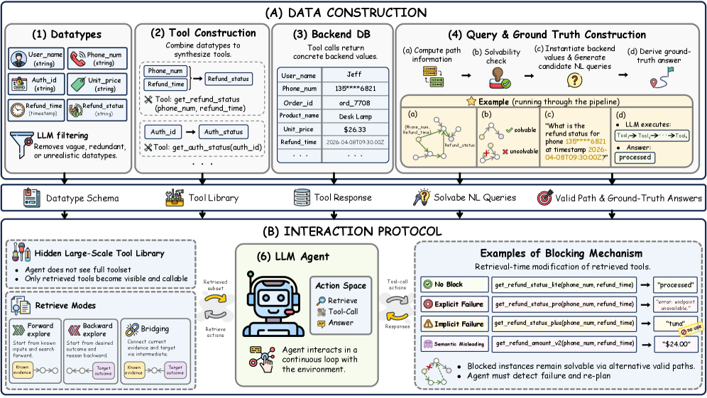
The retriever supports bidirectional exploration: forward (from currently held evidence to tools that consume it) and backward (from target output datatypes to tools that produce them). Tasks are solvable only if the agent stitches together a chain whose intermediate outputs each unlock the next retrieval. The default mode adds retrieval noise; the block mode replaces path-critical tools with corrupted variants (explicit failures, implicit failures, semantic distractions, or mixtures) while guaranteeing solvability through at least one remaining path.
Evaluation protocol
The interaction loop is observe \to reason \to retrieve-or-invoke \to feedback, with T_{\max}=100 turns and a per-retrieval cap \Lambda_{\mathrm{ret}}^{\mathrm{cap}}=30. Metrics cover task completion (Accuracy, Evidence-Grounded Tool Precision), exploration behavior (avg turns, mean Explored Datatypes, Search/Call ratio), and execution quality (Invalid Tool Call Rate, Unused Information Retrieval Rate).
Main results
In the default (no-block) setting under grounded accuracy, Gemini-3.1-Pro leads at 77.06% with EGT precision 91.47%, followed by DeepSeek-V4-Flash at 63.08%, Gemini-3.5-Flash at 52.19%, and GPT-5.4 at 51.90%. Llama-3.3-70B reaches only 18.96%, and several mid-tier open models (Qwen3-8B, Llama-3.1-8B-Instruct) score 0.00%. Notably, GPT-5.4-Mini achieves just 3.07% accuracy with an Invalid Tool Call Rate of 51.71%, indicating schema-violation failure rather than planning failure. The gap between top-tier proprietary models and 70B-class open models exceeds 30 points, suggesting that scale alone is insufficient — typed-schema discipline and retrieval grounding dominate.
Behavior under blocking
The benchmark’s discriminative power emerges under blocking. With block ratio 0.8 (“1 Path”, only one feasible chain remaining), GPT-5.4 collapses to 11.36%, a >40-point drop from its no-block accuracy.
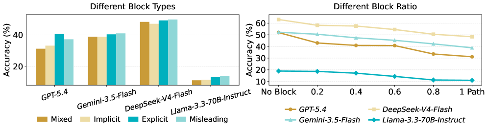
Two patterns stand out. First, implicit failures (tools that return executable-looking but wrong outputs) hurt more than explicit failures (tools that error visibly): agents cannot tell they have drifted off a viable path. Second, accuracy degrades monotonically as the block ratio rises from 0 to 0.8, with GPT-5.4 losing >20 points across the sweep and the same trend replicated across the other three frontier models tested.
Fine-grained blocking that preserves only the longest admissible path is substantially harder than preserving the shortest one, even though both leave the task solvable.
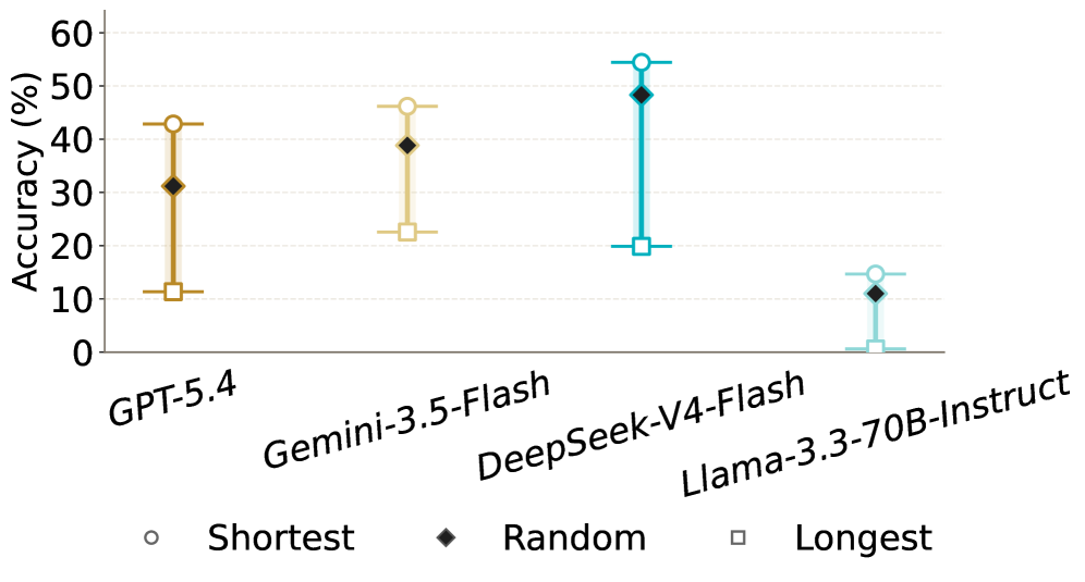
This isolates a specific weakness: agents are not just bad at recovery in general — they are bad at extending plans. When the surviving solution requires more sequential tool invocations, the trajectory drift compounds. Inference-time augmentation via enforced continuation prompts (B_{\mathrm{enf}}\in\{0,\dots,5\} after incorrect termination) recovers only a small fraction of the no-block accuracy, saturating quickly — additional compute does not substitute for correct branch selection.
Error structure
The authors’ three-stage error analysis attributes failures less to retrieval gaps than to selection: the right tool is often in the retrieved set but the agent fails to return to it after a digression. Under blocking, this manifests as the inability to reject misleading-but-executable evidence. Termination behavior diverges by family — some models hallucinate completion, others abort prematurely — but the underlying trajectory breakdown is shared.
Limitations and open questions
The benchmark is single-domain (retail) with LLM-synthesized tools; whether the retrieval-limited planning failures transfer to human-authored APIs with idiosyncratic schemas is untested. The 100-turn budget and 30-tool retrieval cap are generous, so reported numbers are near-optimistic for serving constraints. There is no analysis of training-time interventions (RL on trajectories, schema-aware fine-tuning), so it is unclear whether the gap is fundamentally a capability ceiling or an alignment-of-decoding-to-retrieval problem. Finally, the block-mode design preserves solvability by construction, which may overstate or understate practical recoverability depending on how real ecosystems fail.
Why this matters
PlanBench-XL exposes that frontier LLMs, even those competent in small-tool settings, lose most of their planning accuracy when implicit failures and longer alternative paths are introduced — and that test-time scaffolding does not close the gap. This reframes tool-use evaluation around recovery and re-planning under silent corruption, which is closer to production conditions than current benchmarks.
Source: https://arxiv.org/abs/2606.22388
KaLM-Reranker-V1: Fast but Not Late Interaction for Compressed Document Reranking
Problem
Cross-encoder rerankers (encoder- or decoder-based) score a query–passage pair by jointly encoding the concatenation [q;p], which forces every candidate to be re-processed online at cost \mathcal{O}(KL(|q|+n)^2 d). Late-interaction models (ColBERT-style) separate encoding but reduce interaction to a token-level MaxSim, losing deep cross-attention semantics and inflating storage with one vector per passage token. KaLM-Reranker-V1 targets the middle ground: passage representations should be (i) pre-computable and reusable, (ii) compressible for corpus-scale storage, and (iii) still interact richly with the query at scoring time.
Method
The model is an encoder–decoder initialized from T5Gemma2 at three scales (270M/270M, 1B/1B, 4B/4B activated). The encoder is used offline to map each passage to \mathbf{H}_p = \mathrm{Enc}(p)\in\mathbb{R}^{n\times d}. The decoder, conditioned on system instruction, task instruction I, and query q, attends to the cached \mathbf{H}_p via cross-attention.

Mechanically, the decoder merges self- and cross-attention into a single block by concatenating decoder states with encoder outputs on the key/value side:
\mathbf{Q}=\mathbf{X}\mathbf{W}_Q,\quad \mathbf{K}=[\mathbf{X};\mathbf{H}_p]\mathbf{W}_K,\quad \mathbf{V}=[\mathbf{X};\mathbf{H}_p]\mathbf{W}_V,
with a causal-plus-cross mask \mathbf{M}\in\mathbb{R}^{m\times(m+n)}. The relevance score is the softmax over the two label-token logits at the first prediction position:
\mathrm{score}(q,p)=\frac{\exp(z_{\mathrm{yes}})}{\exp(z_{\mathrm{yes}})+\exp(z_{\mathrm{no}})}.
Matryoshka Embedding Pooling (MEP). To reduce the cost of storing \mathbf{H}_p for a full corpus, MEP mean-pools every r consecutive tokens:
\mathbf{H}_p^{(r)}[j] = \mathrm{MeanPool}\big(\mathbf{H}_p[(j-1)r+1:\min(jr,n)]\big),
yielding \lceil n/r\rceil tokens. Training optimizes a Matryoshka-style sum of SFT losses over \mathcal{R}=\{1,2,4,8,16,32\}:
\mathcal{L}_{\mathrm{sft}}(I,q,p,l,\mathcal{R})=\sum_{r\in\mathcal{R}}\lambda_r\Big(-\log\frac{\exp(z_l^{(r)})}{\exp(z_{\mathrm{yes}}^{(r)})+\exp(z_{\mathrm{no}}^{(r)})}\Big),
so one set of weights supports multiple compression ratios at inference. A knowledge-distillation phase uses a stronger teacher reranker to provide soft labels y\in[0,1] optimized via binary cross-entropy, mitigating false hard-negative noise common in retrieval datasets.

Complexity
With a same-size cross-encoder baseline of L Transformer layers, KaLM’s online decoder is roughly L/2 layers (the rest is offline encoder). Online cost for K candidates is
\mathcal{O}\!\left(\tfrac{L}{2}K\Big(|q|(|q|+\lceil n/r\rceil)d+(|q|+\lceil n/r\rceil)d^2\Big)\right),
versus \mathcal{O}(KL(|q|+n)^2 d + KL(|q|+n)d^2) for joint cross-encoders. For typical |q|=32, n=1024, r=16, d=640, L=36, this is roughly an order-of-magnitude reduction; the quadratic (|q|+n)^2 term collapses to |q|(|q|+n/r) with n/r=64.
Results
On the BEIR subset (13 tasks, top-100 reranked from KaLM-Embedding-V2.5 at avg. nDCG@10 of 53.78):
- KaLM-Reranker-V1-L (4B): 62.87 avg., at 43.7× relative online cost, vs. Qwen3-Reranker-4B at 63.50 but 236.8× cost, and Qwen3-Reranker-8B at 65.11 at 539.7× cost. So KaLM-L gives up ~0.6 nDCG to Qwen3-4B while running ~5.4× cheaper online, and trails the 8B model by ~2.2 nDCG at ~12× lower cost.
- KaLM-Reranker-V1-S (1B): 60.01 avg. at 6.9× cost, beating bge-reranker-large (0.6B) at 51.86 (36.3× cost) and mxbai-rerank-large-v2 (1.5B, 60.32 at 79.2× cost) at a fraction of the compute.
- bge-reranker-v2-gemma (2.5B) reaches only 54.49 at 81.3× cost — KaLM-L is +8.4 nDCG at roughly half the online cost.
Per-task numbers show the gap is largest on retrieval-heavy tasks like FiQA (KaLM-L 62.63 vs. Qwen3-4B 56.69) and QuoraRetrieval (91.00 vs. 88.40); KaLM-L underperforms on ArguAna (74.39 vs. 79.85) and Climate-FEVER (38.56 vs. 49.92), suggesting some domains still benefit from full bidirectional joint encoding.
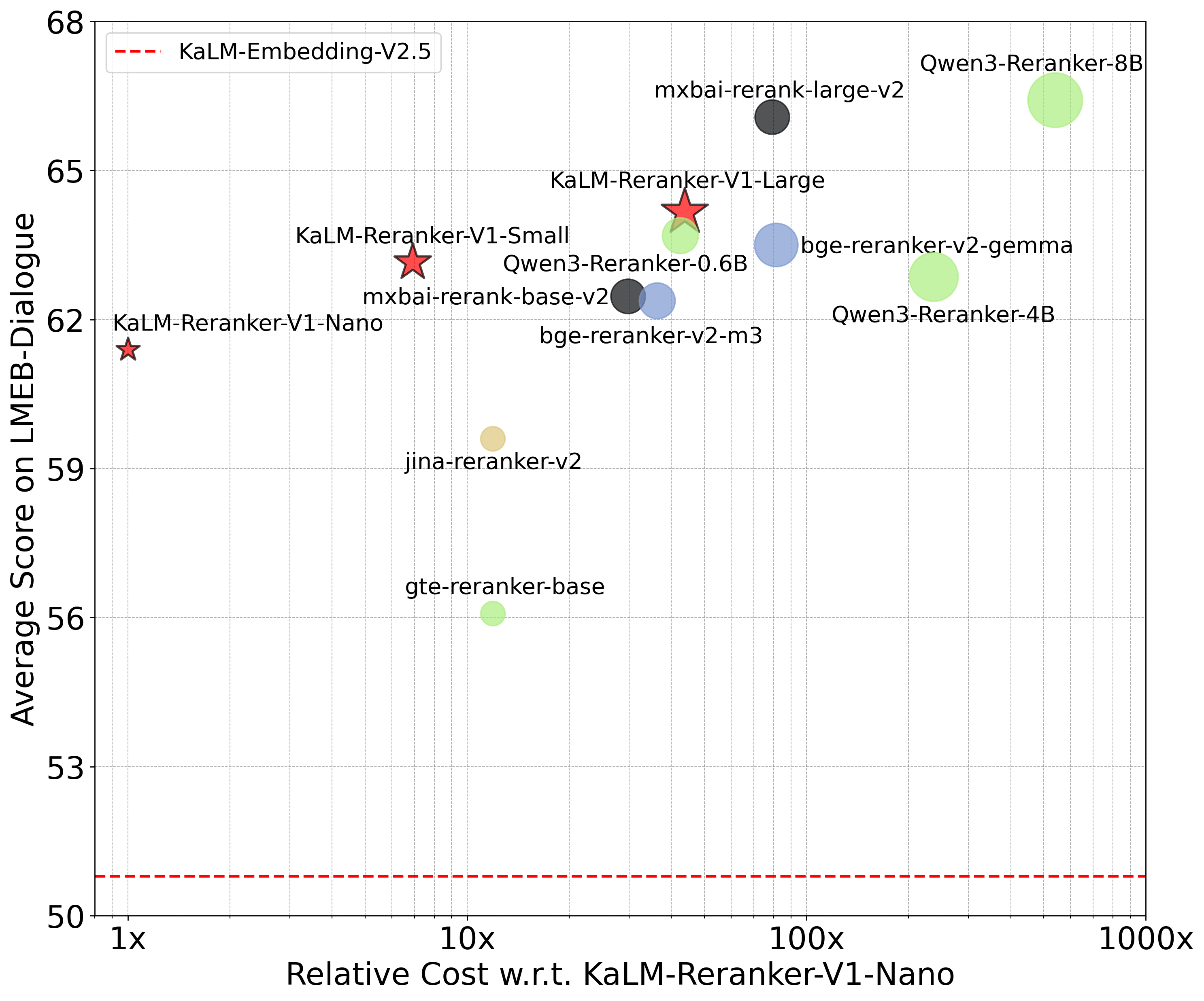
On LMEB-Dialogue, KaLM variants occupy the Pareto frontier of accuracy vs. online cost; this is the regime where pre-cached passage representations matter most because memory documents are reused across many turns.
Limitations and open questions
- Training corpus is “mainly Chinese and English”; MIRACL comparisons are restricted to non-multilingual-trained baselines, so multilingual claims remain partial.
- The 4B model trails 4B/8B cross-encoders in absolute nDCG; whether scaling the decoder (rather than the encoder) closes this gap is untested.
- MEP uses uniform mean pooling. Content-aware pooling, learned downsampling, or query-conditioned pooling could plausibly push the cost/quality frontier further, but the paper sticks with fixed r.
- Storage of \mathbf{H}_p^{(r)}\in\mathbb{R}^{\lceil n/r\rceil\times d} at d=640 is still substantially larger than scalar BM25 or single-vector dense indexes; corpus-scale cost (bytes/passage at various r) is not directly tabulated.
- The “first prediction position” yes/no readout is a single scalar; the architecture admits richer scoring heads that the paper does not explore.
Why this matters
FBNL is a clean architectural point in the rerankers design space: it keeps cross-attention as the interaction mechanism (unlike ColBERT) while paying the encoder cost only once per passage (unlike standard cross-encoders), and Matryoshka pooling makes a single model serve multiple cost/quality operating points. The 5–10× online-cost reductions at near-parity nDCG suggest this is a practical default for large-corpus reranking deployments.
Source: https://arxiv.org/abs/2606.22807
World Action Models: A Survey
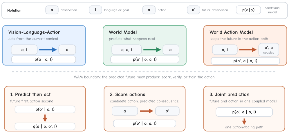
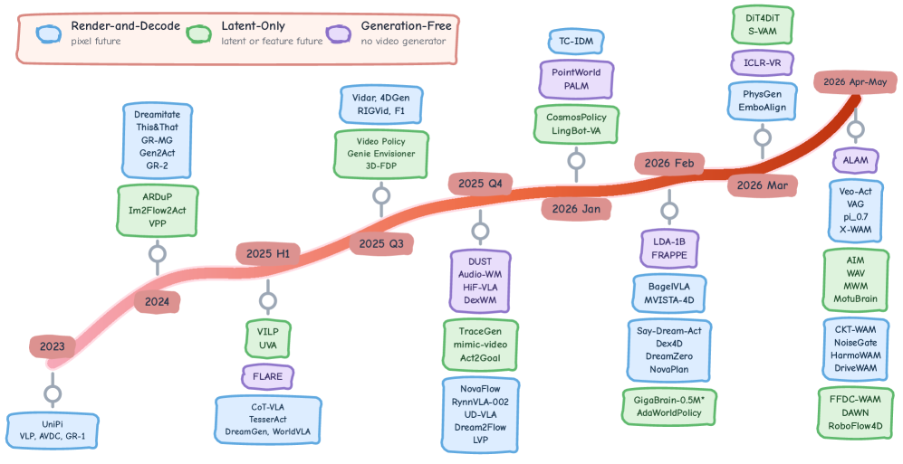
This survey formalizes World Action Models (WAMs) as a distinct class of embodied predictive-action models, separating them from neighbors that are often conflated: Vision-Language-Action (VLA) policies, video world models, and action-grounded video generators. The defining requirement is mechanical: a predicted future observation must remain on the action path — through a cascade (predict-then-act), an action-scoring rollout, or joint future-action prediction.
The boundary against VLAs and video world models
The authors anchor the definition by contrasting the VLA objective
\mathcal{L}_{\text{VLA}}(\theta)=\mathbb{E}_{(o,l,a)}\!\left[-\log p_\theta(a\mid o,l)\right]
with the WAM contract. Equation (1) never requires the model to predict o_{t+1}; RT-2, OpenVLA, and the \pi_0/\pi_{0.5}/\pi_{0.7} family act from the present alone. A model becomes a WAM only when a predicted future “helps produce, choose, or check the action.” Conversely, a vanilla video world model is excluded because its rendered cup-lift is not tied to the controller’s intended trajectory.
Three design philosophies
The taxonomy partitions WAMs by where the action signal is grounded along the inference forward pass, not by training architecture:
- Render-and-Decode: run the video generator to pixels, then extract action (UniPi, AVDC, VLP, Dreamitate, Gen2Act). Cascaded variants (NovaFlow, Dream2Flow, TC-IDM) convert rendered futures into flow, tool trajectories, or inverse-dynamics commands. Easy to bolt onto pretrained video diffusion, but pays full generation cost before any control.
- Latent-Only: video-derived predictor whose decoder is bypassed; action is consumed from intermediate latents, partially denoised features, flow, or value maps.
- Video-Generation-Free: prediction in LLM/VLM token space, JEPA embeddings, regression over frozen vision foundation features, or non-video diffusion over a compact substrate.
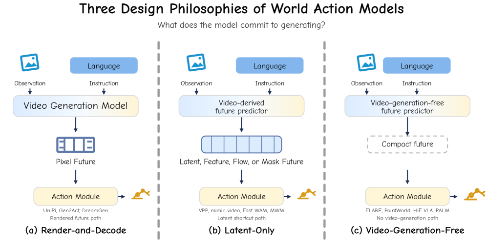
Crucially, this axis is orthogonal to the cascaded-vs-joint distinction: a Latent-Only WAM can be either, and the same holds for Render-and-Decode.
Unified mathematical object
All WAMs are described as a parameterized conditional joint over a future-state window and an action chunk of equal length H:
p_\Theta\!\left(s_{t+1:t+H},\,a_{t:t+H-1}\mid o_{\le t},\,a_{<t},\,l\right). \quad (8)
The substrate space \mathcal{S} — image of an interface encoder \phi:\mathcal{O}\to\mathcal{S} — is the key design variable. Pixel-grounded WAMs expose decoded frames or VAE/VQ grids; feature WAMs expose hidden tokens (frozen SSL teacher targets, VLM future-token blocks); geometric-primitive WAMs expose flow, point clouds, or depth. The four-axis anatomy is then: predictive substrate, action coupling, backbone family, deployment regime.
Action coupling: post-prediction → in-generation → joint
The action-coupling axis is presented as a near-monotone progression in how early the action binds:
- Post-prediction decoding: generate the whole future, then recover control (UniPi, AVDC, VLP; cascaded extensions NovaFlow, Dream2Flow, TC-IDM; Audio-WM for sound).
- In-generation control: This&That conditions diffusion on gesture coordinates; ARDuP restricts conditioning to active regions and decodes from latents; CoVAR and VAG run dedicated action branches alongside video denoising with bridge attention or step-synchronized denoising, passing only pooled video context.
- Joint: UWM, UVA, F1, Motus, and Cosmos Policy share substrate prediction and action heads on a single backbone. AdaWorld binds earliest of all.
Five core properties and their trade-offs
WAMs must satisfy interactability, causality, persistence, physical plausibility, and generalization. The survey is explicit that these are coupled: improving interactability by pushing action earlier into the diffusion stack typically inflates latency or memory; enforcing persistence over long horizons trades against fidelity. WAM design reduces to managing these trade-offs against control-loop budgets.
Data and evaluation
Training data partitions into five groups by the scale/label-fidelity/embodiment-match trade-off: robot teleoperation (Open X-Embodiment, RoboMIND, RoboSet, Human2Robot — clean action labels, expensive), scripted/random robot collection (RoboNet — throughput over precision), plus human video, simulation, and web-scale video (covered subsequently). Evaluation must jointly track visual fidelity, closed-loop success, physical plausibility, and cost; rendered-quality metrics are explicitly insufficient for the control-loop question.
Open challenges: dream more or act more?
The most pointed open question is the fidelity-latency curve. One camp distills or skips video generation: S-VAM distills video diffusion into geometric/semantic features, Fast-WAM removes the future-video branch at inference, GigaWorld-Policy masks attention so future video can be skipped, and X-WAM lets action denoising finish before video denoising. The other keeps imagination in the loop: DreamZero runs a large video backbone in closed loop via custom optimization, CosmosPolicy uses repeated model/value queries, NovaPlan generates video before flow extraction. The authors argue the goal is not smaller models but a controllable fidelity-latency curve, with runtime budget allocated by expected action value — more compute near contact, uncertainty, or irreversible error. DreamAvoid, SANTS, NoiseGate, and HarmoWAM learn this trigger from task phase or denoising state, but a binary execute-or-replan decision is insufficient: the open question is how much of the remaining horizon to regenerate.
The convergence point with mainline video generation is the substrate level of Section 4.2: video generators (Cosmos-Transfer1, cosmos-predict2) add action conditioning while WAMs borrow latent/JEPA substrates from video backbones. A single backbone trained with video objectives, whose action path selects how much of it to run at inference, is identified as the design the field has not yet produced.
Why this matters
By imposing a single mathematical object (Eq. 8) and a three-way taxonomy keyed to where on the inference path action is grounded, the survey converts a fragmented literature into a comparable design space. The fidelity-latency framing — and the empirical observation that the video training objective often matters more than the rendered test-time forecast — points concretely at what the next generation of embodied foundation models should optimize.
Source: https://arxiv.org/abs/2606.20781
Grouped Query Experts: Mixture-of-Experts on GQA Self-Attention
Problem
Standard multi-head attention applies all H heads to every token, regardless of how much that token actually needs. At long context this is doubly painful: attention cost scales as O(n^2) per head, and the per-token head count is fixed by architecture. Grouped-query attention (GQA) already trims the KV side by sharing one KV head across a group of query heads, but the query side stays dense: every query head in every group is computed for every token. The paper asks whether the query side can be made conditionally sparse — a mixture-of-experts over query heads — without losing GQA’s KV-cache benefits or downstream quality.
Method
GQE leaves GQA’s group structure intact and inserts a router inside each group that selects a top-k subset of query heads per token. KV heads remain dense.
Concretely, with H query heads partitioned into G groups (so each group has H/G query heads sharing one KV head), the dense GQA computation is
\text{GQA}(X) = \text{Concat}\big(A_1(X), \dots, A_H(X)\big) W_O,
with each A_h using its group’s shared K_g, V_g. GQE replaces this with a per-token, per-group router r_g(x) \in \mathbb{R}^{H/G} that selects the top-k query heads in group g:
\mathcal{E}_g(x) = \text{TopK}_k\big(r_g(x)\big), \qquad A_h^{\text{GQE}}(x) = \mathbb{1}[h \in \mathcal{E}_g(x)] \cdot A_h(x).
Crucially, K_g, V_g are computed and cached unchanged — so the KV-cache footprint and the KV projection FLOPs are identical to GQA. Only the active query-head projections and the corresponding QK^\top and softmax-weighted V products are sparsified. The output projection W_O multiplies the concatenation with zeros in slots whose experts were not selected for that token.
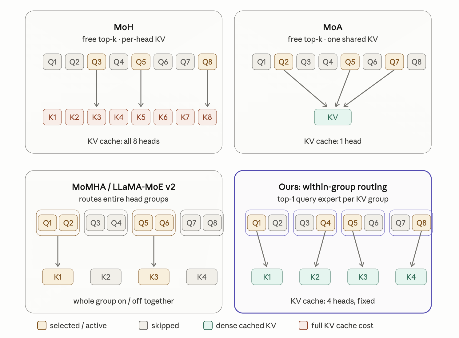
The contrast in the figure is worth dwelling on: prior MoE-on-attention work routes whole heads or whole KV groups, which either breaks GQA’s KV sharing or perturbs the cache. GQE deliberately confines routing to within a GQA group, so each expert’s queries still attend against the same K_g, V_g used by the dense baseline. This makes GQE essentially a drop-in replacement: the only addition is the small router and a top-k mask.
Setup and results
All ablations use a 250M-parameter model trained on a fixed 30B-token sample of FineWeb-Edu, sequence length 2048, batch size 1.05M tokens, fused AdamW (\beta_1=0.9, \beta_2=0.95), WSD schedule with peak LR 5\times 10^{-4}, 3B-token warmup, weight decay 0.1, BF16, and ZClip to handle loss spikes. The baseline is GQA with 8 KV heads (hence G=8); GQE uses the same 8-group layout, with the dense baseline’s query heads serving as the per-group expert pool. In the headline configuration k=1, each group activates one of its query heads per token — halving the active query heads relative to dense GQA when the pool size per group is 2 (the configuration the abstract describes as “half the query heads per token”).
Per-head dimension, tokenizer, optimizer, schedule, and data are held constant across runs so that differences isolate the routing choice rather than head width or training compute.
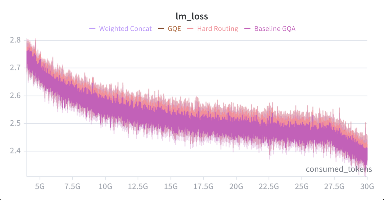
Training loss curves for the variants track the dense GQA baseline closely, with no evidence of the divergence or routing-collapse behavior that has plagued previous attempts at attention-side MoE. Downstream, the authors report HellaSwag, PIQA, and ARC-Easy rather than a single proxy.
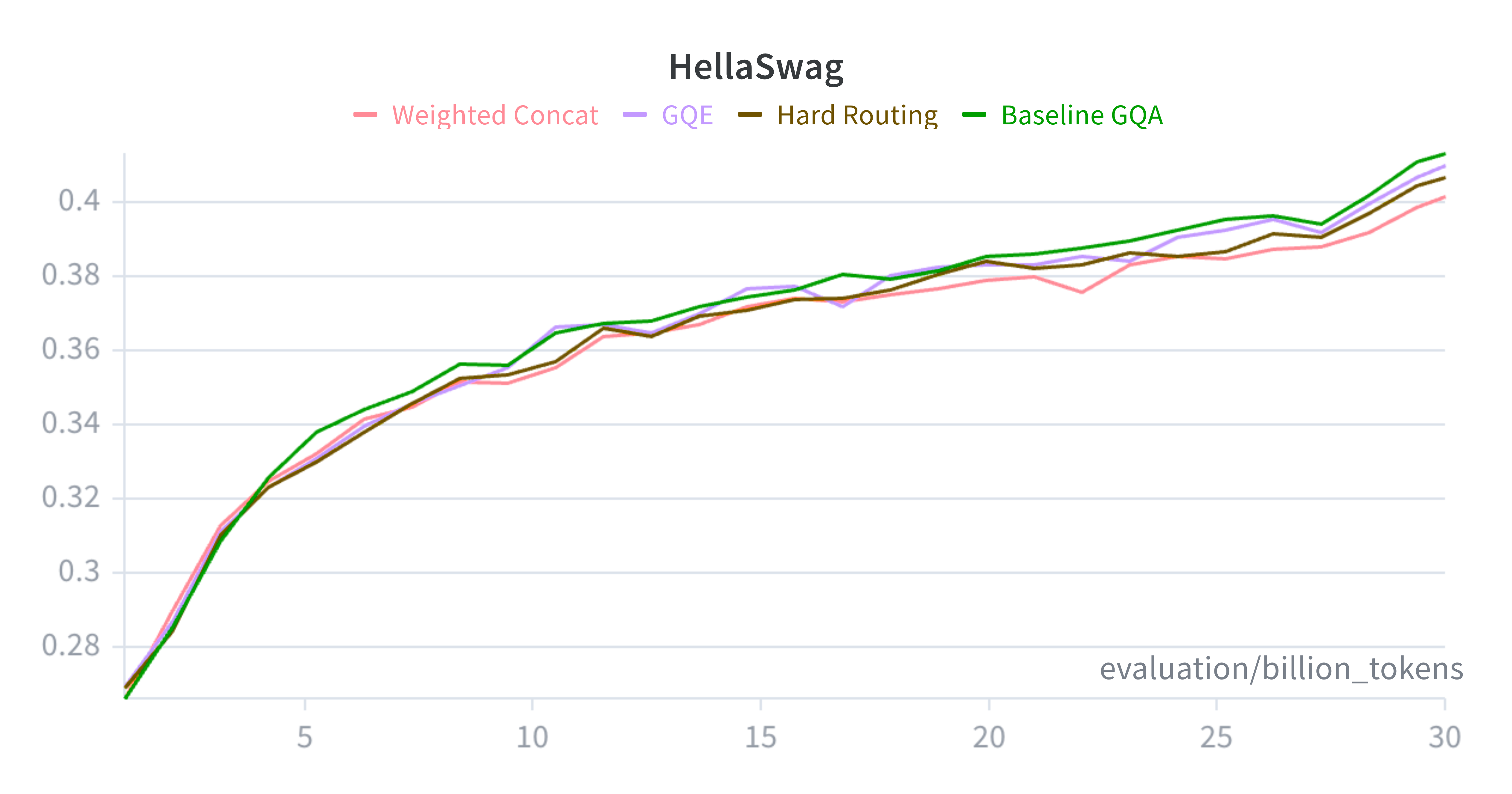
On HellaSwag, the final GQE model matches the dense GQA baseline across the full training trajectory, despite activating half the query heads per token. The paper’s central claim — parity on downstream accuracy at the 30B-token, 250M-parameter scale with halved active query-head compute — is supported by this curve plus the corresponding PIQA and ARC-Easy numbers (reported in their Table 2). Throughput is reported as a function of context length, since the savings are largest where attention dominates the FLOP budget.
Limitations and open questions
The evaluation is at a single scale (250M params) and a single token budget (30B). It is unclear whether parity holds at 1B+ scale, where attention’s relative cost shrinks compared to MLPs and where router-induced load-balancing pathologies typically emerge. The paper’s k=1 setting halves query heads only if each group has exactly two experts; the scaling law in expert pool size per group is not characterized. No auxiliary load-balancing loss formulation is described in the provided sections, and the practical wall-clock speedup depends on whether sparse top-k head dispatch can be made efficient on modern GPU kernels (dense attention kernels are highly tuned; sparse-head variants typically lose constants). Finally, the KV path remains dense, so GQE does not help with the KV-cache bottleneck that dominates long-context inference memory.
Why this matters
GQE shows a clean way to apply conditional computation to the query side of attention without breaking the GQA KV-sharing contract that production LLMs already depend on. If the parity result holds at larger scales, it offers a near-free reduction in attention FLOPs that composes with — rather than competes against — the existing GQA/MQA stack.
Source: https://arxiv.org/abs/2606.20945
EvoEmbedding: Evolvable Representations for Long-Context Retrieval and Agentic Memory
Problem
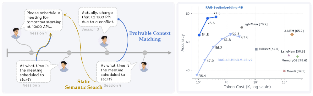
Dense retrievers encode each segment in isolation: \mathbf{v}_t = f(x_t). This is fundamentally mismatched with agentic memory and long-context personalization, where the correct target for a query depends on conversational state that has evolved over hundreds of segments. The same query (“what is my current address?”) should retrieve different facts depending on which segments preceded it. Existing approaches either (a) concatenate context into the encoder, blowing up cost and exceeding context windows, or (b) build external memory pipelines (Mem0, A-Mem, MemoryOS) that require explicit LLM-driven summarization, paying substantial token overhead.
Method
EvoEmbedding maintains a recurrent latent memory \mathbf{M}_{t-1} \in \mathbb{R}^{C \times D} that is updated as segments stream in, and conditions every embedding on that memory. Two LoRA adapters share the same base LLM:
\mathbf{\tilde{M}_t} = \pi_{\theta_m}(x_t, \mathbf{M}_{t-1}), \qquad \mathbf{v}_t = \pi_{\theta_r}(x_t, \mathbf{M}_{t-1}).
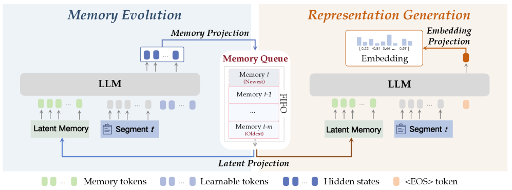
Both passes prepend a projection of the previous memory to the segment tokens: \tilde{x}_t = [m_{in};\, x_t;\, r_l] where r_l are K=16 learnable tokens for memory evolution, replaced by <EOS> for retrieval. The memory pass reads the last K hidden states; the retrieval pass reads the <EOS> hidden state and projects it to D_{emb}=1024.
Latent memory queue. Rather than caching layer-wise KV (as in M+), EvoEmbedding stores a FIFO queue of C = L \times K = 512 tokens:
\mathbf{M}_t = \text{Queue}(\mathbf{M}_{t-1},\, f_m(\mathbf{\tilde{M}_t})).
The bounded loop L is critical: each historical memory is recurrently re-encoded at most L times, which the authors argue prevents the representation collapse documented in prior recurrent-encoder work and removes the need for curriculum learning on context length. Memory footprint is roughly that of one encoded image.
Dynamic segment-batching. Sequential segment processing is the obvious efficiency bottleneck. The authors batch k consecutive segments — chosen so concatenated length stays under 2048 tokens — and share the same \mathbf{M}_{t-1} across them: \mathbf{\tilde{M}}_{t:t+k} = \pi_{\theta_m}(x_{t:t+k}, \mathbf{M}_{t-1}). This is technically an approximation (segments in the batch don’t see each other’s intermediate memory updates), but it yields a reported 3.8x training speedup. The memory is only advanced one step per batch, which is the principal limitation of this trick.
EvoTrain-180K. 184,137 instances with context lengths up to 10,270 tokens and up to 246 segments per sample (mean 20.57). Each instance has on average 19.45 contrastive negatives; queries are short (mean 15.59 words). 52.9% of samples are under 512 tokens, with a long tail — the mixed-length design is what lets the model generalize from 10K-token training to 128K-token inference on PersonaMME.
Results
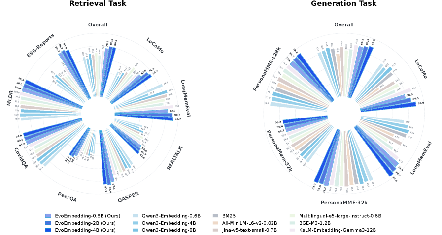
Evaluation spans 10 benchmarks: retrieval (ESG-Reports, MLDR, CovidQA, PeerQA, QASPER), conversational memory retrieval (REALTALK, LoCoMo, LongMemEval), and generation/personalization (LoCoMo, LongMemEval, PersonaMem-32K, PersonaMME-32K/128K). Baselines include Qwen3-Embedding, BGE-M3, multilingual-e5, BM25, plus agentic memory systems Mem0, LightMem, A-Mem, MemoryOS, and reranking pipelines (Qwen3-Reranker-4B).
Headline claims from the abstract and Figure 1/2:
- EvoEmbedding family (0.8B, 2B, 4B) outperforms larger static embedding models across all 10 benchmarks, with the largest margins on dynamic-context tasks like long-term personalization.
- Standard RAG using EvoEmbedding-4B beats specialized memory architectures (Mem0, LightMem, A-Mem, MemoryOS) on LongMemEval, while consuming zero tokens for explicit memory construction — the memory lives in \mathbf{M}_t, not in prompt-side text.
- The model trained only with contexts up to ~10K tokens generalizes to 128K-token PersonaMME, attributed to the mixed-length distribution and the bounded-loop guarantee.
- Segment-batching delivers 3.8x training acceleration.
Default config: C=512, K=16, D_{emb}=1024, 8x H800.
Limitations and open questions
The paper does not (in the provided sections) quantify how performance degrades when the true relevant segment is older than L memory steps — the FIFO is a hard forgetting mechanism, and 512 latent tokens is a tight bound for 500+ segment conversations. The segment-batching approximation effectively makes memory update granularity coarse during training; the trade-off curve between k and final retrieval accuracy is not shown here. Recurrent inference precludes parallel embedding of independent segments, which matters for cold-start indexing of large corpora. Finally, evaluations use Qwen3-30B-A3B as generator and GPT-4o-mini as judge; the judge dependency is a known confound for memory-system comparisons.
Why this matters
Treating an embedding as a function of streaming state rather than of an isolated chunk is the right architectural move for agentic memory, and EvoEmbedding shows that a bounded latent queue plus dual LoRA adapters is sufficient to beat both larger static encoders and explicit memory-construction pipelines without paying their token cost. If the bounded-loop claim holds at larger L, this is a practical drop-in replacement for the embedding layer in RAG-based memory agents.
Source: https://arxiv.org/abs/2606.21649
Hacker News Signals
Moebius: 0.2B image inpainting model with 10B-level performance
Moebius is a compact image inpainting model that claims competitive quality with models 50x its size. The core technical contribution is a two-stage architecture that separates structure prediction from texture synthesis. In the first stage, a small transformer predicts a coarse structural completion of the masked region, conditioned on surrounding context. In the second stage, a diffusion-based refinement network fills in texture details, using the structural prediction as a conditioning signal rather than raw pixel context alone.
The key insight is that large inpainting models spend most of their capacity learning structure-texture co-occurrence statistics that can be factored apart. By giving the texture stage an explicit structural prior, the model avoids needing deep representations to infer geometry from pixels alone. The structural predictor is trained with a masked autoencoding objective over a latent space; the texture diffusion model is a standard DDPM-style network conditioned on both the structural tokens and the visible image context.
Benchmark comparisons on Places2 and COCO inpainting tasks show FID and LPIPS scores matching or beating several 5B-10B parameter baselines. At 0.2B parameters the model is fast enough for interactive use on consumer hardware.
The interesting open question is how much of the performance gap to larger models is truly closed versus being masked by benchmark-specific saturation. Inpainting metrics notoriously fail to capture semantic coherence in complex scenes, and the cherry-picked qualitative results on the project page show simpler backgrounds. Generalization to heavily occluded faces or dense urban scenes with strong perspective constraints is not thoroughly evaluated.
Why this matters
Demonstrates that architectural factoring — separating structural from textural generation — can substitute for raw parameter scale, which has practical implications for on-device deployment of generative image tools.
Source: https://hustvl.github.io/Moebius/
VibeThinker: 3B param model that beats Opus 4.5 on reasoning with novel SFT+GRPO
VibeThinker trains a 3B-parameter reasoning model using a two-phase pipeline: supervised fine-tuning (SFT) on a curated chain-of-thought dataset, followed by Group Relative Policy Optimization (GRPO), a variant of PPO that avoids a separate value network by computing advantages relative to a group of sampled responses for the same prompt.
The GRPO objective normalizes rewards within a batch of K completions per prompt, computing the advantage as A_i = (r_i - \bar{r}) / \sigma_r where r_i is the scalar reward for completion i, \bar{r} is the group mean, and \sigma_r is the standard deviation. This eliminates the need to train a critic, reducing memory overhead substantially and making RL fine-tuning tractable at small parameter counts.
The SFT stage uses a filtered mix of mathematical reasoning and logical puzzle data, prioritizing examples where intermediate steps are verifiable. The GRPO stage then uses outcome-based rewards (final answer correctness) without process reward models, keeping the pipeline simple.
Reported results show scores on AIME 2024, MATH-500, and LiveCodeBench that exceed Claude Opus 4.5 on several tasks, though the comparison methodology deserves scrutiny: frontier models are typically evaluated with much more inference compute, and the benchmark overlap with training data for small models is a persistent concern.
The architecture base is not clearly specified in the abstract (the paper lists it as a “3B reasoning backbone”), which makes reproduction harder. The claim of beating Opus on reasoning is plausible in narrow benchmark ranges but the evaluation breadth is thin.
Why this matters
Demonstrates that GRPO-based RL fine-tuning can transfer strong reasoning to sub-5B models cheaply, which matters for edge deployment and for researchers who cannot afford frontier API calls.
Source: https://arxiv.org/abs/2606.16140
The text in Claude Code’s “Extended Thinking” output is not authentic
Patrick McCanna argues that the extended thinking tokens surfaced to users in Claude Code do not represent the model’s actual internal reasoning process. The post is grounded in a specific technical observation: when Claude Code operates in extended thinking mode, Anthropic’s API returns a thinking block alongside the final response. The argument is that this block is not a raw transcript of intermediate computation but is instead a post-hoc or constrained generation artifact — effectively a rationalization narrative rather than a causal trace.
The evidence cited is behavioral: the thinking text can contradict the final answer, appear to reason toward a wrong conclusion before the response is correct, and shows stylistic uniformity inconsistent with unconstrained scratch-pad generation. There is also the architectural point that transformer inference is a single forward pass per token; there is no separate “reasoning substrate” from which text is extracted. The thinking tokens are generated autoregressively from the same weights and sampling process as the response, just with a different system prompt or sampling configuration.
This is consistent with what is publicly known about chain-of-thought: CoT tokens improve downstream accuracy through prompt conditioning effects, but they are not mechanistically privileged traces of computation. The model is not “checking its work” in any sense that maps onto human metacognition.
The practical implication for developers using Claude Code is that the thinking block should be treated as a soft hint about the model’s uncertainty or approach, not as an auditable reasoning log. Debugging based on thinking-block output can be misleading if the block rationalizes the wrong answer rather than exposing why the error occurred.
Why this matters
Directly relevant to AI interpretability assumptions embedded in developer tooling; conflating generated rationalization with causal inference traces leads to incorrect debugging strategies.
Source: https://patrickmccanna.net/the-text-in-claude-codes-extended-thinking-output-is-not-authentic/
GLM-5.2 – How to Run Locally
GLM-5.2 is THUDM’s latest release in the GLM series, and the Unsloth documentation covers quantized local deployment. The technical substance here is in the inference stack rather than the model architecture itself.
Unsloth’s approach applies 4-bit and 8-bit GPTQ/GGUF quantization to GLM-5.2, reducing VRAM requirements substantially. The GLM architecture uses bidirectional attention in certain prefix positions (inherited from earlier GLM designs), which complicates naive quantization relative to purely causal models — attention masks interact with quantization calibration data in non-trivial ways. Unsloth handles this by calibrating on mixed-prefix sequences representative of the model’s actual use patterns.
The documentation covers setup via ollama, llama.cpp, and direct Python inference through the transformers library with bitsandbytes backends. GLM-5.2 uses a rotary positional embedding variant and a specific tokenizer that differs from standard BPE setups common in Llama-family models, so model loading requires the THUDM tokenizer rather than a generic one — a common source of silent failures in community deployments.
GLM-5.2 is notable for strong Chinese-English bilingual capability and competitive coding benchmark scores relative to its size class. The quantized 4-bit version reportedly runs on a 24GB consumer GPU at reasonable throughput for interactive use.
The main open issue is that GGUF conversion of GLM-5.2 required patches to llama.cpp due to the non-standard attention pattern, and those patches are not yet merged upstream as of the documentation’s publication, meaning users need to track a specific fork.
Why this matters
Practical deployment friction for non-Llama architectures remains high; this documentation surfaces the specific patching and calibration steps needed to run attention-variant models locally.
Source: https://unsloth.ai/docs/models/glm-5.2
Good results fine tuning a local LLM like Qwen 3:0.6B to categorize questions
This post documents a concrete fine-tuning experiment on Qwen 3 0.6B for a classification task: routing educational questions into categories. The setup uses Unsloth for memory-efficient LoRA fine-tuning, targeting the attention projection matrices with rank-16 adapters, which keeps the trainable parameter count well under 1% of total weights.
Training data was ~500-1000 labeled examples constructed manually, which is at the lower edge of what LoRA fine-tuning typically needs for stable convergence on a constrained classification problem. The author reports near-perfect accuracy on held-out examples, which is plausible for a low-cardinality classification task with clear category definitions.
The technically interesting observation is that 0.6B models, despite weak zero-shot classification performance, respond well to even small amounts of task-specific fine-tuning for narrow problems. This is consistent with the hypothesis that small models have adequate capacity for classification but lack the in-context instruction following to express it reliably. LoRA fine-tuning essentially bypasses the instruction-following bottleneck by directly adjusting the decision boundary.
The post also notes that structured output (forcing JSON via constrained decoding) improved consistency further, which is a useful practical point: for classification, combining fine-tuning with grammar-constrained generation eliminates the class of errors where the model produces a correct answer in an unparseable format.
Limitations: the evaluation is informal (no held-out test set with rigorous splits), and the dataset size is too small to know whether performance generalizes to question phrasings outside the training distribution.
Why this matters
Demonstrates the practical viability of sub-1B models for production classification tasks via LoRA plus constrained decoding, relevant for privacy-sensitive or low-latency edge deployments.
Source: https://www.teachmecoolstuff.com/viewarticle/fine-tuning-a-local-llm-to-categorize-questions
The new HTTP QUERY method explained
The HTTP QUERY method is an IETF draft standardizing a request method for safe, idempotent queries that carry a request body. It addresses the fundamental mismatch in existing HTTP semantics: GET cannot carry a body by spec, POST is not idempotent and cannot be safely cached, and GET-with-body is technically undefined and rejected by many intermediaries.
The mechanical specification: QUERY is defined as safe (no side effects) and idempotent, exactly like GET, but explicitly permits a request body. The response semantics are equivalent to GET — caching intermediaries can treat QUERY responses as cacheable using the same cache key logic, with the request body as part of the cache key. This is the critical piece: existing POST workarounds for body-carrying queries cannot be cached by default because POST is not defined as safe, so CDNs and proxies discard those responses.
This has concrete implications for GraphQL deployments (which send queries as POST bodies, breaking CDN caching), search APIs, and any endpoint that accepts complex filter or aggregation specifications too large for a URL. The QUERY method lets these use cases get full HTTP caching semantics without hacks like GET-tunneling over POST.
Implementation requires explicit support in HTTP servers, clients, and intermediaries. The draft is at a mature stage but not yet an RFC. Kreya (the app behind this post) has implemented client-side support, which is why they wrote the explainer.
The open question is adoption timeline: even once standardized, CDN and proxy support will lag, and existing API clients default to the GET/POST dichotomy, so actual use will take years to normalize.
Why this matters
Fills a genuine gap in HTTP semantics that has caused real architectural compromises in API design and caching for over a decade.
Source: https://kreya.app/blog/new-http-query-method-explained/
Linux and Secure Boot certificate expiration (2025)
The LWN article covers an operational problem in the Linux Secure Boot chain: the Microsoft-signed UEFI certificate used to verify Linux bootloaders (specifically the Shim layer used by most distributions) has an expiration date, and the revocation and renewal process for Secure Boot signing chains is non-trivial.
The technical structure is: UEFI firmware trusts a Microsoft root certificate, Microsoft signs a key enrollment key (KEK), Shim is signed by Microsoft and embeds a distribution-specific key, and the distribution key signs GRUB and the kernel. Expiration or revocation at any level breaks the chain. The current issue involves the intermediate signing infrastructure rather than the root, but the resolution path requires coordinated updates to Shim, DBX (the revocation database stored in UEFI firmware), and MokManager entries on deployed machines.
The practical problem is that DBX updates are delivered via Windows Update for machines that dual-boot, and not all firmware vendors ship DBX updates reliably. Linux-only machines with older firmware may not receive DBX updates at all, requiring manual intervention via efi-updatevar or equivalent tools.
There is also a subtler issue: rotating Secure Boot signing keys for bootloaders requires that all currently deployed kernels and bootloaders either remain trusted or get re-signed, which is operationally complex for distributions supporting long-term releases. The interaction between MOK (Machine Owner Key) enrollment and the system DBX state is poorly understood by most system administrators.
Why this matters
Certificate hygiene in the Secure Boot chain is often invisible until a system fails to boot post-update; this is a real operational risk for Linux deployments, especially in environments with locked-down firmware.
Source: https://lwn.net/Articles/1029767/
Show HN: Oak – Git alternative designed for agents
Oak is a version control system designed around the assumption that agents (automated code-modifying processes) are the primary committers, not humans. The design diverges from Git in several ways motivated by agent use patterns.
The core data model replaces Git’s DAG of snapshots with an explicit operation log — a sequence of typed operations (file create, file modify, file delete, rename) rather than tree diffs. This makes merging agent-generated changes cheaper because common agent operations (append to file, insert at line) can be represented as commutative or order-independent operations where possible, reducing conflicts. Git’s blob-diff merge is line-oriented and does not understand operation semantics.
Oak also redesigns branching around task isolation rather than human feature branches. Each agent task gets a lightweight “workspace” (analogous to a branch but with stricter isolation semantics and automatic cleanup on merge). The locking model is per-file optimistic concurrency rather than Git’s whole-repository lock-free model, which avoids the class of conflicts where two agents modify the same file simultaneously in incompatible ways by surfacing the conflict immediately rather than at merge time.
The storage backend is content-addressable like Git’s object store, so deduplication properties are preserved. The CLI surface is smaller than Git’s by design, omitting operations that are rarely needed by automated workflows.
The project is early-stage and self-hosted on Oak itself (the repo URL is the Oak instance). The main open questions are: whether the operation-log model scales to large repositories with high agent commit frequency, and whether the semantics handle the full diversity of real agent modification patterns beyond simple append/insert.
Why this matters
Version control semantics were designed for human cognitive patterns; as agent-driven development scales, the mismatch with Git’s merge model will become a real bottleneck.
Source: https://oak.space/oak/oak
Noteworthy New Repositories
myccarl/ai-shortVideo-pipeline
An end-to-end pipeline for automated short-video production, combining a FastAPI orchestration layer with a Spring Boot API gateway. The architecture implements multi-model failover so that if a primary generative model (video, TTS, music) is unavailable, a circuit breaker routes to a secondary without manual intervention. Metering hooks track per-model token and compute costs across the pipeline run.
The quality-gating layer is the more interesting engineering piece. Prompt anchoring ensures that downstream generation steps remain semantically consistent with the original brief. CLIP consistency checks compare generated frames against a reference embedding to catch visual drift. AV sync auto-rescue detects audio-video misalignment and triggers re-rendering or offset correction rather than failing the job entirely. Full-stack observability is wired in via structured logging and trace IDs propagated across both the Python and JVM layers.
Pick this if you need a production-grade skeleton for agentic video workflows rather than a research demo. The multi-service boundary (FastAPI + Spring Boot) matches teams that already split Python inference from Java/Kotlin service infrastructure.
Source: https://github.com/myccarl/ai-shortVideo-pipeline
SantanderAI/gen-fraud-graph
A synthetic fraud graph generator targeting reproducible benchmarks for graph-based fraud detection in financial services. The core problem it solves is data scarcity: real transaction graphs are proprietary and cannot be shared, making benchmark comparison across institutions nearly impossible.
The generator produces labeled directed graphs where nodes represent entities (accounts, merchants, devices) and edges represent transactions. Fraud subgraph patterns — structurally distinguishable motifs such as mule chains, ring networks, and layering cycles — are injected at configurable prevalence rates. Edge and node features (transaction amounts, timestamps, categorical merchant codes) are sampled from parameterizable distributions intended to approximate empirical statistics without leaking real data.
The output format is compatible with standard graph-ML tooling (NetworkX, PyG, DGL), so plugging a GNN baseline in is straightforward. Seed control and reproducible generation make it suitable for ablation studies comparing GCN, GraphSAGE, and heterogeneous graph transformer approaches on a fixed benchmark.
Primary limitation: the statistical properties of the synthetic graphs are manually specified rather than learned from real data, so distributional realism depends on how carefully the generator is calibrated. Still, for teams without access to internal fraud data, this provides a controlled evaluation harness.
Source: https://github.com/SantanderAI/gen-fraud-graph
cobusgreyling/loop-engineering
A framework and CLI toolkit for designing human-in-the-loop and agent-to-agent orchestration patterns with AI coding agents, drawing on ideas from Addy Osmani’s agent-loop writing and Boris Cherny’s structured agent design work.
The three main CLI tools define the surface area: loop-init scaffolds a new agent loop project with opinionated directory structure and config; loop-audit statically analyzes an existing loop definition for common failure modes (unbounded recursion, missing exit conditions, absent human-escalation hooks); loop-cost instruments a loop run and reports estimated token and API costs per step, which matters when loops can run hundreds of iterations.
The patterns library covers prompt-chaining loops, reflection loops (agent critiques its own output before proceeding), and multi-agent debate structures. Each pattern ships as a composable starter rather than a black-box abstraction, so the internals remain readable and modifiable.
Targeted at engineers building autonomous coding workflows — CI bots, refactor agents, test-generation pipelines — where loop reliability and cost predictability matter more than raw capability.
Source: https://github.com/cobusgreyling/loop-engineering
sums001/Windows-Copilot-API
A reverse-engineered wrapper that exposes Windows Copilot as an OpenAI-compatible REST API, allowing access to GPT-4 and reportedly GPT-5 class models without direct API keys or billing. The interface mirrors the /v1/chat/completions endpoint schema, so existing clients using the OpenAI SDK can point at this server with a base URL change and no other modification.
The technical work involved intercepting the HTTP(S) traffic between the Windows Copilot client and Microsoft’s backend, identifying session token handling, and wrapping that into a local proxy server. Authentication reuses the ambient Windows session credentials rather than an API key.
Practical use cases are narrow: local development and experimentation where the user already has a licensed Windows environment. Reliability depends entirely on Microsoft not rotating the underlying protocol, making this unsuitable for anything production-facing. Rate limits from the consumer-facing Copilot service apply and are not documented publicly.
This is useful primarily as a reference for protocol reverse-engineering methodology and for researchers wanting to probe model behavior without managing API billing during exploratory work. Treat it as brittle infrastructure.
Source: https://github.com/sums001/Windows-Copilot-API
datalab-to/lift
A document-to-structured-data extraction library focused on accuracy and throughput. The core abstraction is a typed schema definition against which arbitrary documents (PDFs, scanned images, HTML, plain text) are parsed, with the output being validated JSON conforming to that schema.
Under the hood, Lift combines layout-aware document parsing with LLM-driven field extraction, using the document’s visual and semantic structure to ground extraction rather than treating the input as a flat text stream. This matters for documents like invoices, contracts, and forms where spatial relationships carry meaning that pure text serialization loses.
The library exposes a Python API where you define an extraction schema as a Pydantic model (or equivalent dataclass), pass a document, and receive structured output with per-field confidence scores. Batch processing and async support are included for pipeline integration.
What differentiates it from generic LLM prompting for extraction is the layout-grounding step, which reduces hallucination on documents with dense tabular content or multi-column layouts. Compared to heavier OCR + NLP pipelines (e.g., LayoutLM fine-tuning), it trades some accuracy ceiling for ease of deployment — no GPU required.
Source: https://github.com/datalab-to/lift
Tejas-TA/predikit
A bridge library for exposing trained ML models as tool-callable functions consumable by AI agents (LangChain, LlamaIndex, custom function-calling workflows). The central problem: most ML model interfaces are designed for batch offline inference, not for low-latency synchronous tool calls from an LLM agent.
Predikit wraps sklearn, XGBoost, LightGBM, and PyTorch models behind a unified Predictor interface that handles input validation, feature preprocessing, and output serialization to agent-readable formats. A decorator-based API lets you annotate existing model-serving code with schema metadata — feature names, types, expected ranges — that gets surfaced as a JSON Schema tool description for the agent.
The framework also handles prediction explanation: SHAP values can be optionally computed and returned alongside predictions, letting an agent reason about why a fraud score is high or a churn probability elevated, rather than just acting on the scalar output.
This fills a genuine gap: MLflow, BentoML, and similar tools target human-facing APIs or batch jobs, not the sub-200ms synchronous call pattern that agent tool use demands.
Source: https://github.com/Tejas-TA/predikit
Nigh/show-me-the-story
A self-hosted long-form fiction generator distributed as a single Go binary with an embedded web UI. The architecture is intentionally minimal: no external database, no container orchestration. Configuration points at any OpenAI-compatible API endpoint (local Ollama, remote OpenAI, etc.).
The generation pipeline is structured rather than a single long-context prompt. The system first constructs an outline (acts, chapter summaries, character arcs), then writes chapters iteratively. After each chapter, a review pass checks for internal consistency, flags unresolved foreshadowing threads, and runs a lightweight fact-check against established world-state. A final full-book polish pass runs after all chapters are complete, targeting continuity and tonal consistency.
Bilingual support (Chinese and English) is first-class, with prompt templates and review heuristics tuned for both languages — not simply a language parameter passed through.
The Go binary distribution is the practical differentiator: writers who are not engineers can run this on a laptop without installing Python environments or managing dependencies. The codebase is readable enough to serve as a reference for multi-stage LLM pipeline design in Go.
Source: https://github.com/Nigh/show-me-the-story
saiyam1814/kiac
A local Kubernetes setup that runs on Apple’s native container virtualization framework (introduced in macOS 15), where each Kubernetes node runs in its own lightweight VM rather than sharing a single VM as tools like Minikube do. This more closely mirrors production multi-node cluster topology on a laptop.
The tooling provisions a full multi-node cluster using Apple’s containerization framework, which leverages the Virtualization.framework directly for low-overhead VMs. Each node gets isolated networking, and the setup includes metrics-server for kubectl top functionality, persistent storage provisioning, and a LoadBalancer implementation (likely backed by a local proxy) so LoadBalancer type services work without external cloud dependencies.
This is relevant for testing workloads that require node-level failure simulation, DaemonSet behavior, pod anti-affinity across real nodes, or network policy enforcement between nodes — scenarios that single-node local clusters cannot accurately reproduce. It targets Apple Silicon Macs specifically, where the virtualization overhead is low enough to make running three or four VMs simultaneously practical.