Daily AI Digest — 2026-06-17
arXiv Highlights
LoopCoder-v2: Only Loop Once for Efficient Test-Time Computation Scaling
Problem
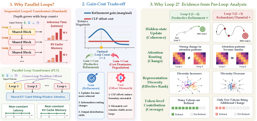
Looped Transformers reuse a shared block R times to grow effective depth without adding parameters, but standard sequential looping inflates inference latency and KV-cache memory linearly in R. Parallel Loop Transformers (PLT) sidestep this by giving each loop a cross-loop position offset (CLP) and a shared-KV gated sliding-window attention (G-SWA, window w=64), so the loops execute against a single cache and loop count becomes a near-free design knob. The natural question is then: how many loops should you pay for? The authors show empirically that the answer is “one extra,” and explain mechanistically why deeper loops actively hurt.
Setup
All experiments use a 7B dense PLT with G-SWA (w=64) and first-loop KV sharing applied uniformly across loops. Four variants are pretrained from scratch on 18T tokens with R \in \{1,2,3,4\} (baseline, PLT_2, PLT_3, PLT_4), followed by matched instruction tuning so only R varies.
Macroscopic result: strongly non-monotonic in R
PLT_2 improves SWE-bench Verified from 43.0 to 64.4 (+21.4) and Multi-SWE from 14.0 to 31.0 (+17.0) over the R=1 baseline. The same model hits 33.4 on the held-out agentic SWE-bench-CC, putting a 7B dense model above 30B–72B open models and within range of 480B-class systems on Verified. PLT_3 and PLT_4, despite seeing more latent compute, regress and frequently fall below the R=1 baseline. The curve peaks sharply at R=2.
Microscopic diagnostics
The authors instrument hidden-state geometry across loops: step size \delta^{(r)} = \lVert h^{(r)} - h^{(r-1)} \rVert, angular change \cos\theta^{(r)}, effective rank \mathrm{erank}(h^{(r)}), and a fixed-point gap \Delta_{\text{FP}}^{(r)}.
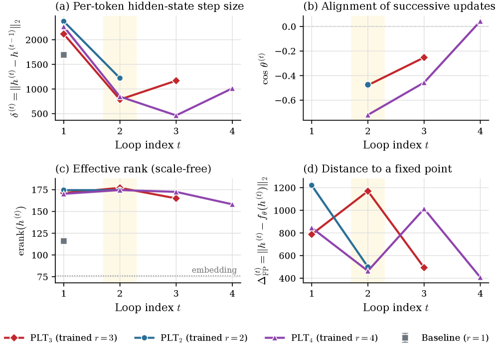
Several signatures converge on the same picture. Effective rank peaks at r=2 and declines monotonically thereafter, so deeper loops collapse representational diversity rather than expand it. Successive updates are oscillatory (\cos\theta^{(r)}<0) through the refinement loops — the model overshoots and partially undoes prior updates — and \delta^{(r)} shrinks to a mid-depth minimum before rebounding at the readout loop, the rebound being decoding rather than new computation. The fixed-point gap does not contract, so the loop is not behaving as a contractive iterative solver.
Output-side lenses tell a consistent story. The per-loop output-distribution shift \Delta p^{(r)} = D_{\mathrm{KL}}(p^{(r-1)} \,\|\, p^{(r)}) collapses after r=2 and never recovers; the logit-lens ground-truth rank still sharpens with depth, but mostly via output readout, not fresh refinement. Inter-loop attention KL drops sharply after loop 2, i.e., attention routing freezes; per-head cosine similarity grows across loops, indicating heads degenerate into redundant copies. The G-SWA gate weighting the global loop-1 branch stays above 0.5 at every loop, meaning later loops mostly re-read the same first-loop KV through a narrow local window.
The gain–cost scissors
The paper’s central quantitative explanation is a per-loop accounting of refinement gain \Delta p^{(r)} against the intrinsic CLP offset cost \Omega^{(r)} (their Eq. 6), which measures the positional mismatch CLP injects at each loop boundary.
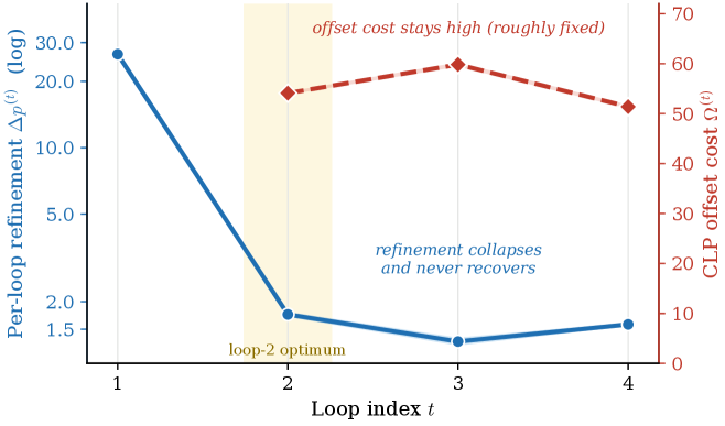
\Omega^{(r)} is approximately loop-invariant — it is a fixed property of the offset scheme — while \Delta p^{(r)} decays by orders of magnitude after r=2. At every loop r \geq 3, the offset cost exceeds the refinement gain by 30–45x. This is a clean structural argument: the CLP “tax” is amortized only when there is meaningful representational work left to do, which on this architecture is exhausted by loop 2. Decomposing post-context refinement across r \geq 2 for PLT_4 under three independent lenses (output shift, attention re-routing, per-token peak contribution) all assign the dominant share to loop 2.
Limitations and open questions
The analysis is tied to one architecture (G-SWA w=64, first-loop KV sharing, this particular CLP scheme) and one scale (7B, 18T tokens). The conclusion that “one extra loop” is optimal is conditional on \Omega^{(r)} being roughly constant; alternative position-handling schemes that decay the offset cost with r, or that adapt CLP per loop, could move the optimum. The fixed-point gap not closing suggests PLT is not implementing iterative inference in the Deep Equilibrium sense, leaving open whether a contractive parameterization could rescue R \geq 3. Finally, the diagnostics are correlational; no intervention shows that artificially zeroing \Omega^{(r)} recovers gains at loop 3.
Why this matters
For test-time scaling of small models, this work argues that latent looping has a sharp, identifiable optimum that can be predicted from a gain–cost decomposition rather than searched empirically — and that for current PLT designs, the answer is R=2. The 43.0 → 64.4 jump on SWE-bench Verified at fixed parameter count is a concrete demonstration that disciplined latent depth, not more loops, is what pays.
Source: https://arxiv.org/abs/2606.18023
Show the Signal, Hide the Noise: Spectral Forcing for Pixel-Space Diffusion
Problem
Pixel-space diffusion denoisers are trained on inputs whose useful information is highly non-uniform across frequency. Under rectified flow z_t = t x + (1-t)\varepsilon with natural-image power-law spectra S(k)\propto k^{-\alpha}, the per-band data-to-noise ratio crosses unity at a moving cutoff
k^{\ast}(t) \;=\; (1-t)^{-2/\alpha},
separating a low-frequency signal-bearing wedge from a high-frequency band where the Bayes-optimal denoiser collapses to a deterministic baseline (zero-prediction or pass-through). A standard pixel-space denoiser must rediscover this boundary internally at every t, spending capacity on regions where there is no data-distribution structure to learn. This matters because pixel-space DiTs (e.g., JiT) avoid VAEs precisely to keep modeling end-to-end, but then pay this hidden capacity tax — particularly under coarse tokenization where each token must summarize a wide spectral band.
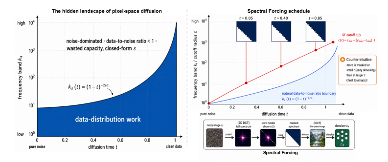
Method
Spectral Forcing (SF) is a parameter-free, time-conditional 2D-DCT low-pass operator inserted before the patch embedder. Given z_t, SF computes the 2D-DCT, zeroes coefficients with radial frequency above a cutoff k_c(t), and inverts. The cutoff schedule f(t) = k_c(t)/k_{\max} expands monotonically with t and reaches identity at t=1, so the data endpoint is unmodified. Two schedules are studied:
- Linear: f(t) = t.
- Analytical: f(t) = \max(c_{\min}, (1-t)^{-2/\alpha}/k_{\max}), tracking the theoretical contour with a floor c_{\min} to keep DC-region tokens populated early.
Training is unchanged otherwise: rectified-flow velocity loss \mathcal{L} = \mathbb{E}\|v_\theta(z_t,t,y) - (x-\varepsilon)\|^2, logit-normal time sampling \mathcal{N}_{\text{logit}}(-0.8, 0.8), Heun-50 sampler, CFG 2.9. SF is purely an input-side mask; it adds no parameters and no FLOPs to the backbone.
The motivating diagnostic is per-band \log_{10}(\mathrm{MSE}_{\text{net}}/\mathrm{MSE}_{\text{zero}}) on the (t,k) plane. In a 1D toy and on a trained JiT-700M/32, three regions emerge: a low-k recovery wedge (network beats zero-prediction), a high-k noise-dominated band where the network ties the closed-form baseline, and the transition aligned with k^{\ast}(t).
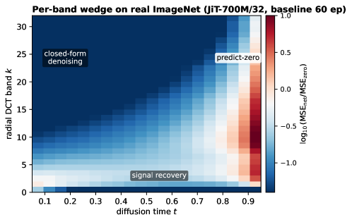
The wedge transfers from synthetic data to real ImageNet, validating that the implicit boundary the model must learn is the explicit boundary SF imposes.
Results
All numbers are FID-50k on ImageNet-256, averaged over 5 seeds, with same-recipe baselines.
Coarse tokenization (64 tokens, p=32). SF improves FID at every (model, epoch) pair tested. The headline is JiT-700M/32 at 60 epochs: 24.19 \to 20.68 (+14.5%). At 90 ep: 19.90 \to 17.53 (+11.9%); at 120 ep: 16.46 \to 15.15 (+8.0%). For JiT-130M/32: +11.6% at 15 ep (114.03 \to 100.78), compressing to +0.4% at 100 ep and +1.5% at 200 ep.
Two regimes for training budget. At small scale (130M/32) most of the gain is data-efficiency — the unforced baseline closes the gap. At large scale (700M/32) a meaningful asymptotic component remains: SF at 120 ep (FID 15.15) matches the prior best 700M+ reference at ~145 ep (FID 15.24).
Schedule. Linear SF (+14.5%) beats Analytical SF with c_{\min}=0.20 (+9.3%, FID 21.94) at the headline, despite the analytical schedule winning by 2–3× in the h=64 toy. The analytical-wins ordering returns at higher resolution.
Patch-size / token-count sweep at JiT-130M, 60 ep:
| p | Tokens | Base | +SF | \Delta |
|---|---|---|---|---|
| 16 | 256 | 21.76 | 21.29 | +2.2% |
| 32 | 64 | 44.68 | 42.92 | +3.9% |
| 64 | 16 | 84.50 | 84.69 | −0.2% |
The favorable regime is bounded on both sides; the operative axis is token count, not patch size or resolution alone.
Resolution. At 512^2 with p=32 (256 tokens), SF recovers a +3.4% FID margin (68.34 → 66.01) where the same token count at 256^2 was neutral. In toys, analytical-SF moves from worst at h=64 to −15% at h=256, saturating at −3.3% by h=512.
Hidden costs at fine tokenization. At JiT-130M/16, 60 ep, Analytical-SF (c_{\min}=0.20) ties baseline on FID (21.23 vs 21.76, +2.4%) but loses 6.6% Inception Score (78.04 vs 83.59) — class-diversity collapse masked by FID. Linear-SF here is benign (FID 21.29, IS 83.13).
Data structure (toys). On power-law data SF is data-efficiency only; on structured data the analytical schedule wins because the front tracks the true noise-dominated bands; on rectangle data both schedules fail because high-frequency edge content carries essential signal — the controlled analogue of the 256-token regime.
Limitations and open questions
- The operator is regime-bounded: it is helpful only when patchification already throws away little usable high-frequency content, i.e., \leq 64 tokens at 256^2 or proportionally at higher resolution. At fine tokenization it can degrade IS without moving FID.
- Schedule choice is empirical: Linear beats Analytical on real ImageNet at 64 tokens despite the analytical schedule’s theoretical alignment with k^{\ast}(t). The authors note this reverses with resolution but offer no principled selection rule.
- \alpha is treated as a global constant; class- or region-conditional spectra are not exploited.
- All evaluation is FID/IS on ImageNet-256/512; no likelihood or perceptual-quality numbers are reported, and no scaling beyond 700M.
Why this matters
SF identifies a concrete capacity-allocation pathology in pixel-space diffusion — denoisers wasting parameters rediscovering the moving signal/noise boundary k^{\ast}(t) — and fixes it with a parameter-free, FLOP-free DCT mask that yields up to 14.5% FID improvement at 700M scale. It is a clean argument that the right inductive bias for pixel-space DiTs is spectral, not architectural, and gives a recipe to close part of the gap with latent-space models without a VAE.
Source: https://arxiv.org/abs/2606.15236
Rethinking the Role of Efficient Attention in Hybrid Architectures
Hybrid architectures interleaving full attention with efficient mixers (SWA, Mamba-2, GDN, Lightning) are now standard, but the literature treats efficient-attention choice as a capability lever — assuming larger receptive fields or more expressive recurrences yield better long-context behavior. This paper challenges that framing through a controlled scaling study, mechanistic probes, and architecture ablations, arguing that efficient attention is best understood as an optimization prior rather than the substrate of long-range retrieval.
Setup
The authors compare a full-attention baseline (Full) against six 1:1 layer-wise hybrids: SWA-128, SWA-512, SWA-2048, and recurrent variants Lightning, Mamba-2, GDN. Five model scales S1–S5 (15M to 477M non-embedding params, hidden 384–1280, GQA with 2 KV heads) are trained, with scaling laws fit jointly for validation \mathrm{Loss} and \log(\mathrm{LongPPL}).
Scaling: convergence in the limit, divergence in the transient
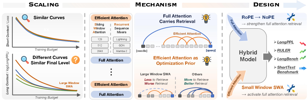
Short-context \mathrm{Loss} curves of all hybrids overlap closely with Full across D, consistent with prior work. The interesting signal is in \log(\mathrm{LongPPL}): at low data budgets, hybrids differ substantially, but the curves converge as D grows.
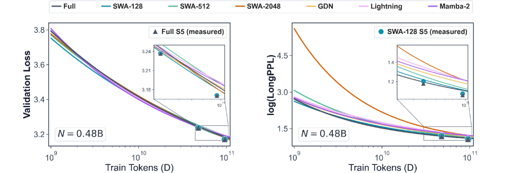
The implication is that efficient-attention design controls how fast long-context capability emerges, not the asymptote it reaches. Larger SWA windows and unbounded-receptive-field recurrences do not yield better long-context performance once training is sufficient — they merely change the trajectory.
Mechanism: full attention does the retrieval
A receptive-field restriction experiment at S4 with D=1000N isolates which module actually carries long-range information at inference. Each module is independently capped at \approx 2048 tokens.

Restricting full attention sharply raises \log(\mathrm{LongPPL}) across all hybrids; restricting efficient attention is nearly a no-op — even for GDN and Mamba-2, whose recurrent state is in principle unbounded. In other words, the recurrent states do not store retrievable long-range content in this regime; full-attention layers do. Layer-wise probing (deferred to Appendix D) corroborates this.
This explains “Large-Window Laziness”: with SWA-2048, full-attention layers can free-ride on the local-context capacity provided by the wide window, delaying the formation of dedicated retrieval heads. Smaller SWA windows force full-attention layers to specialize earlier, accelerating long-context emergence even though the asymptotic capability is similar. The efficient module thus shapes the optimization landscape rather than supplying retrieval capacity.
Design implications
Given that full attention does the heavy lifting, the natural intervention is to strengthen it directly rather than tune the efficient module.
Layer ratio. A 1:3 (full:efficient) variant of SWA-128 matches 1:1 in \mathrm{Loss}, and lags only at small scales in \log(\mathrm{LongPPL}); the gap closes as N grows. Full-attention density can be reduced once a sufficient absolute number of full-attention layers is present.
NoPE on full-attention layers only. Applying NoPE to just the full-attention layers of an SWA-128 hybrid (positional encoding retained on SWA layers for locality) yields large downstream gains. At S4 (0.22B, D\approx 100B), 16K evaluation:
- Full: RULER 25.09, RULER NIAH 35.95, LongBench 15.09
- SWA-128: 35.33 / 49.58 / 15.88
- SWA-128-NoPE: 44.80 / 67.81 / 16.43
At S5 (0.66B), 32K evaluation:
- Full: RULER 43.90, NIAH 62.61, LongBench 18.93
- SWA-128: 41.86 / 60.17 / 18.30
- SWA-128-NoPE: 46.98 / 70.42 / 19.46
Short-context averages over 19 benchmarks are essentially unchanged (S5: Full 40.46, SWA-128 41.31, SWA-128-NoPE 41.32). The +20-point RULER NIAH jump at S4 from removing positional encoding on the small set of full-attention layers is striking and aligns with the mechanism: SWA layers handle locality, and unfettered (positionally unconstrained) full attention does retrieval more effectively.
Limitations and open questions
The largest model is 0.66B at D\approx 100B; convergence claims rest on extrapolated scaling laws, and “sufficient training” is not characterized in compute-optimal terms. All hybrids use a 1:1 baseline ratio with alternating placement; placement strategies (e.g., front-loaded full attention) are not compared. The mechanistic claim that recurrent states “store little long-range information” is specific to this training regime — Mamba-2/GDN may behave differently with longer training contexts or different state sizes. Finally, the NoPE result interacts with extrapolation behavior; it is unclear how it composes with explicit length-generalization techniques like YaRN or with longer pretraining contexts.
Why this matters
The paper reframes hybrid design: efficient-attention modules are optimization priors, not long-context substrates, and the lever for long-context capability is the full-attention path itself. The simple SWA-128 + NoPE-on-full-only recipe delivers concrete gains (RULER NIAH 65.91 → 82.31 at 0.66B/16K) without short-context regressions, suggesting current hybrids over-invest in efficient-module sophistication and under-invest in full-attention configuration.
Source: https://arxiv.org/abs/2606.15378
Looped World Models
Problem
World models for long-horizon simulation face a depth/cost trade-off: faithful multi-step rollouts require deep computation to approximate iterated dynamics, but stacking layers inflates parameter count and amplifies compounding error across rollouts. The paper proposes Looped World Models (LoopWM), which replace stacked transformer depth with iterated application of a single parameter-shared block, framing latent depth as an orthogonal scaling axis to width and data.
Method
LoopWM is a latent dynamics model with four modules: an observation encoder \mathcal{E}_\phi producing e_k = \mathcal{E}_\phi(o_k) \in \mathbb{R}^d, a looped transition core, an action conditioning path, and decoders for observation/reward/termination. The core idea is that a single transformer block f_\theta is applied T times to a latent z_k^{(0)} initialised from (e_k, a_k):
z_k^{(t+1)} = f_\theta\!\left(z_k^{(t)};\, a_k\right), \quad t = 0, \dots, T-1,
with the final z_k^{(T)} serving as the predicted next latent state. Because f_\theta is shared across iterations, total parameter count is decoupled from effective depth: doubling T doubles compute but not parameters. This is the source of the claimed up-to-100x parameter efficiency.
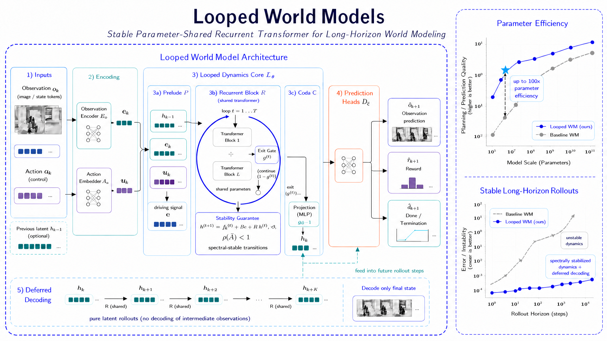
The authors emphasise three design principles: (i) structural alignment between iterative computation and the iterative nature of physical dynamics — the loop count T acts as an internal “simulation step” budget separate from the environment step k; (ii) provable stability of the latent recurrence across arbitrary rollout lengths, which the paper argues follows from constraints placed on f_\theta to keep the iterated map contractive (the section heading promises a stabilised core, though the formal Lipschitz/contraction conditions are not reproduced in the excerpt); and (iii) adaptive computational depth via early exit at inference: a halting predictor decides per-step when z_k^{(t)} has converged, so easy transitions terminate after a few iterations while hard ones use the full T. This yields per-transition compute that scales with predicted complexity rather than worst-case depth.
Training combines next-state prediction with the standard observation/reward/termination decoding losses, plus a regulariser on the halting distribution to prevent collapse to either t=1 or t=T. The action enters the loop at every iteration (rather than only the input), which is what distinguishes this from a generic looped transformer applied to dynamics.
Results
The main evaluation is on ScienceWorld (Wang et al., 2022), feeding five consecutive actions and scoring the final predicted world state with EM, token F1, BLEU-4, and entity metrics. With ~1B parameters, LoopWM reports overall EM 68.4%, F1 85.3%, BLEU-4 80.7%, entity 83.9%, versus claude-opus-4-6-max at EM 47.2%, F1 72.8%, BLEU-4 64.4%, entity 72.3% — a 21.2 EM point gap against a closed-source model the authors claim is >100x larger. Per-task gains are uneven but large where they exist: Lifespan goes from 0% to 100% EM, Conductivity from 47.8% to 87.0%, Boil from 22.2% to 66.7%, Incline EM from 34.0% to 59.3% (with F1 95.3% vs 86.5%). LifeStages is degenerate for both models (0% EM). Smaller baselines qwen-3.5-flash and gemini-3-flash-preview-thinking score overall EM 10.0% and substantially below LoopWM across the board.
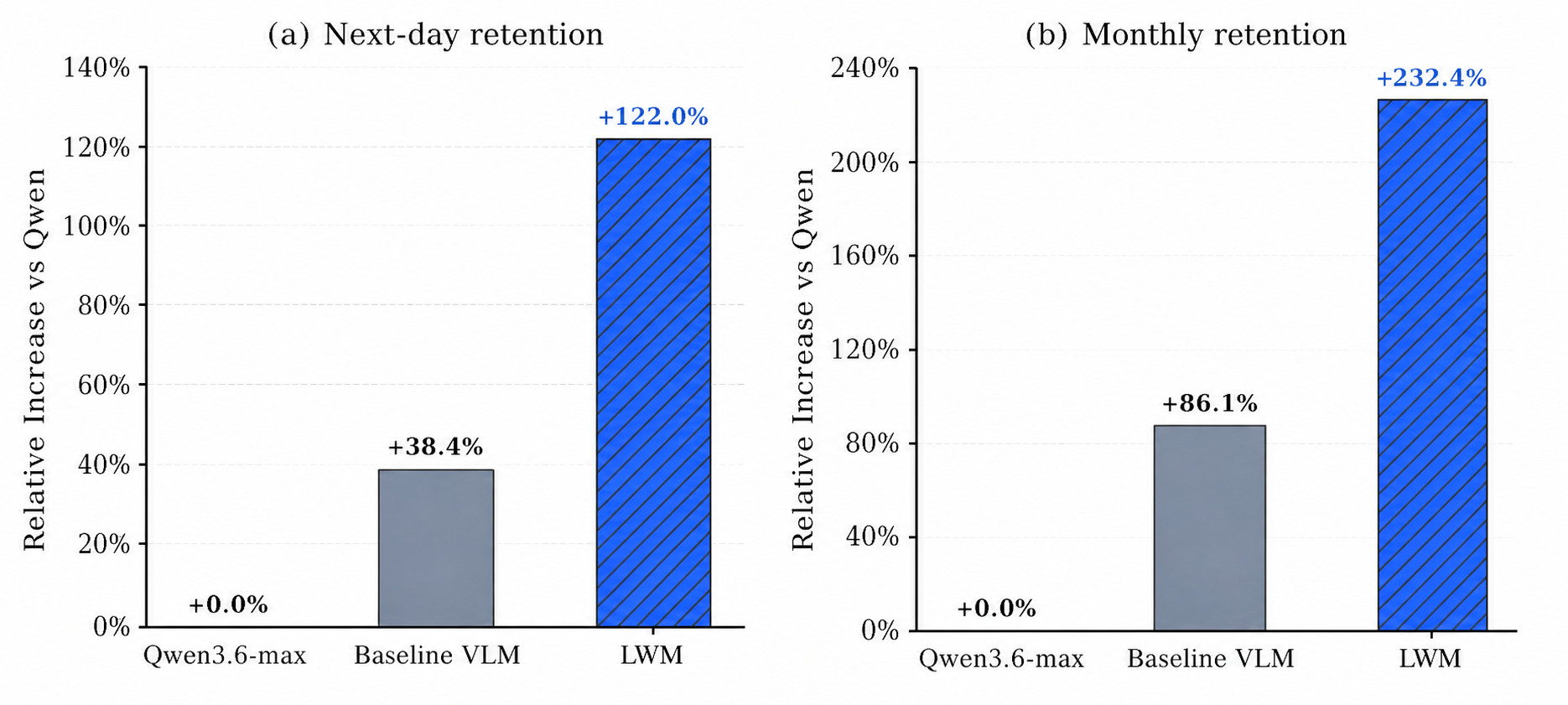
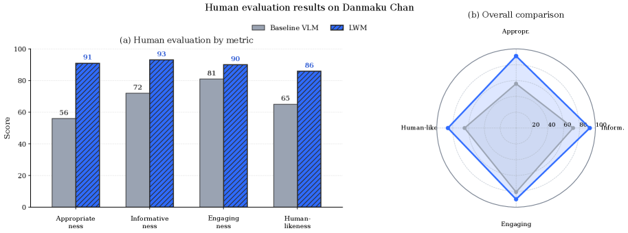
Online evaluation on a danmaku generation task (Figure 2) shows LoopWM’s relative improvement over the Qwen3.7-max reference exceeds the other baselines. Human evaluation (Figure 3) corroborates this on the same task.
Limitations and open questions
The paper as excerpted leaves several technical points unresolved. The “provable stability” claim is asserted but the contraction argument and its assumptions on f_\theta are not given in the provided sections; without those, the claim that error does not compound across long rollouts is unsupported. The headline parameter-efficiency comparison is against an API model whose true size and architecture are unknown, so the “100x” figure is a lower bound at best and conflates parameter count with capability. The held-out tasks where LoopWM underperforms (LifeStages 0% EM, Freeze 25% EM) suggest the looped core does not uniformly handle all dynamics classes — possibly tasks requiring symbolic reasoning over long temporal scopes that the halting predictor under-allocates iterations to. There is no reported ablation in the excerpt isolating (a) loop count T, (b) early-exit vs fixed depth, or (c) parameter sharing vs an unrolled equivalent, all of which are needed to substantiate “iterative latent depth as a scaling axis.” The ScienceWorld setup uses only 5-action rollouts, which is short relative to the long-horizon claim. Finally, the cited references include works dated 2025–2026, and the arXiv ID 2606.18208 is anomalous; readers should verify provenance.
Why this matters
If the stability and adaptive-depth claims hold under proper ablation, parameter-shared iteration becomes a credible third scaling axis for world models alongside width and data, with concrete deployment implications: a 1B model that matches or exceeds frontier API models on structured simulation tasks would change the cost calculus for model-based RL and planning.
Source: https://arxiv.org/abs/2606.18208
Zone of Proximal Policy Optimization: Teacher in Prompts, Not Gradients
Problem
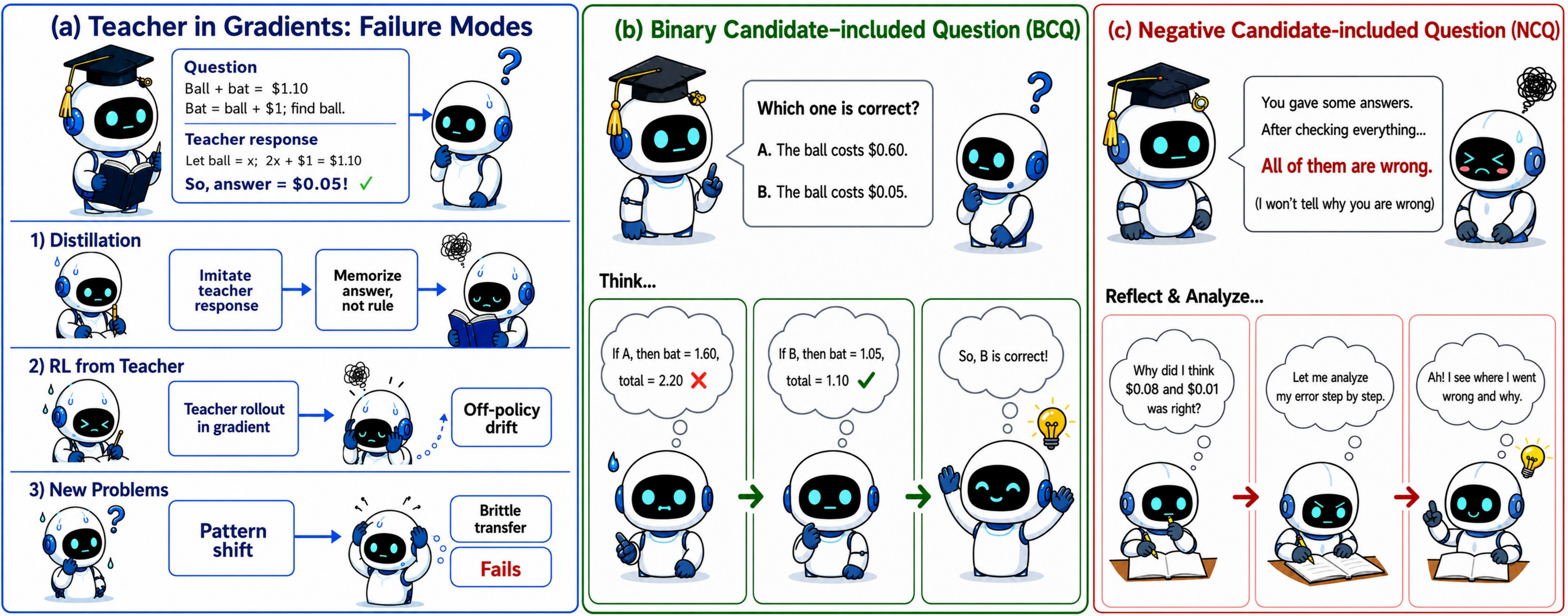
Distilling a strong teacher into a small student is brittle in two complementary ways. Logit-level KD over-concentrates the student on the teacher’s sharpest modes, hurting OOD generalization. RL with verifiable rewards (GRPO-style) sidesteps this by training on the student’s own rollouts, but inherits a sharp blind spot: when all G_S rollouts for question x fail, \bar{r}_x=0, so the group-relative advantage
A^{(g)} = \frac{r(x,y_S^{(g)}) - \bar{r}_x}{\mathrm{std}_x + \epsilon}
is identically zero and the question is silently dropped. Precisely the questions a small student cannot yet solve — the ones a teacher could most help with — contribute zero gradient. A naive fix, splicing a teacher trajectory y_T into the gradient as if it were on-policy, induces distributional drift since y_T \not\sim \pi_\theta.
Method
ZPPO, named after Vygotsky’s zone of proximal development, keeps the teacher in the prompt context rather than in the policy gradient. The student still updates only on its own rollouts; the teacher merely reshapes the questions on which the student now generates.
A question is declared hard when \bar{r}_x < 0.5. The threshold is not arbitrary: under \{0,1\} rewards, \mathrm{std}_x is maximized at \bar{r}_x=0.5, so the strongest learning signal lives just below the hard/easy boundary; pushing the boundary toward 0.5 from below is exactly where ZPPO’s intervention has highest marginal value.
Two prompt reformulations recover signal on hard x:
- BCQ (Binary Candidate-included Question). Take one correct teacher response y_T^+ and one incorrect student rollout y_S^-, anonymize and shuffle them, and reformulate x as a discrimination task: “given these two candidate solutions, which is correct?” The student now generates a fresh chain-of-thought to discriminate; its rollouts again carry \{0,1\} rewards but the task is dramatically easier than open-ended solution, so \bar{r}_x moves off zero and A^{(g)} becomes informative. The teacher’s content sits in the prompt — never in the loss.
- NCQ (Negative Candidate-included Question). Aggregate multiple wrong student rollouts \{y_S^{(g)-}\} into a single prompt asking the student to identify the shared failure mode and produce a corrected solution. No teacher tokens are needed; the structure forces the model to attend to its own systematic errors.
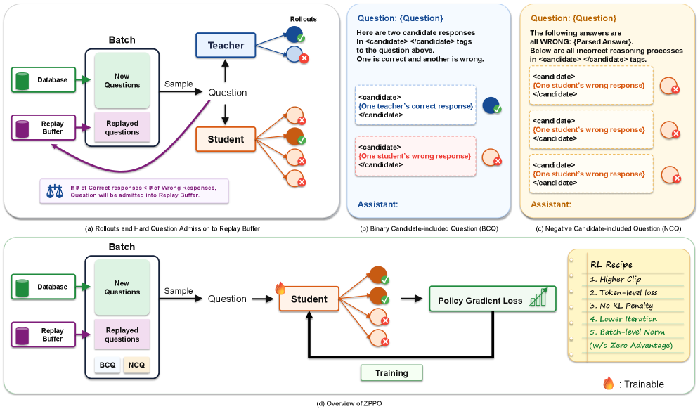
A prompt replay buffer admits hard questions and re-emits their BCQ/NCQ variants over subsequent steps, amplifying their effect since each hard x may need multiple exposures to graduate (i.e., reach \bar{r}_x \geq 0.5 on the original form). The advantage estimator is the two-step REINFORCE++ variant: subtract per-group mean, then batch-normalize across non-trivial groups, plugged into the standard PPO clipped surrogate. Algorithmically the change relative to GRPO is local: a hard-question detector, two prompt-rewriting functions invoking the teacher only at admission time for BCQ, and a buffer that re-injects reformulated prompts into subsequent training batches.
Results
The authors instantiate ZPPO on Qwen3.5 at 0.8B, 2B, 4B, and 9B student scales with a 27B teacher, post-training each as a VLM on a 77K multimodal RL dataset.
The clearest mechanistic evidence is the graduation curve at 2B: cumulative count of admitted-then-graduated hard questions versus their entry rollout accuracy, comparing ZPPO to GRPO augmented with the same replay buffer. ZPPO graduates substantially more hard questions, and the gap widens as entry accuracy approaches zero — exactly the regime where vanilla GRPO sees zero advantage and the buffer alone cannot help.
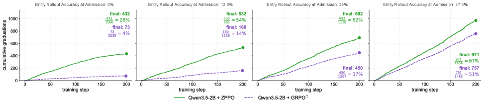
This isolates the contribution of BCQ/NCQ from the contribution of replay: the buffer alone cannot rescue all-wrong groups because the gradient is still zero; reformulation is what turns those questions into trainable instances.
Limitations and open questions
The reward is correctness-only (rule-based exact match plus LLM-as-judge for free-form items); ZPPO targets reasoning competence, not safety or fairness, and inherits Qwen3.5 pretraining biases. BCQ requires teacher access for at least one correct response per admitted hard question, so the teacher cost scales with the hard-set size; NCQ is teacher-free but presupposes that the student’s wrong rollouts are diverse enough for failure-mode aggregation to be informative. The \bar{r}_x < 0.5 threshold is justified by std-maximization but never swept. Anonymization of BCQ candidates relies on length/style not leaking provenance — an empirical assumption worth probing, since a small student could short-circuit discrimination by detecting teacher style rather than reasoning. The graduation metric is reported at 2B; per-scale graduation dynamics and the BCQ-vs-NCQ ablation are not surfaced in the excerpts shown here.
Why this matters
ZPPO offers a clean separation between where the teacher’s information enters (the prompt, off-gradient) and what drives the update (the student’s own rollouts, on-policy). That decoupling addresses the precise pathology that makes RLVR fail on small students — the all-wrong group — without re-introducing the off-policy drift that teacher-trajectory injection creates, and it does so with a small, drop-in modification to GRPO-style pipelines.
Source: https://arxiv.org/abs/2606.18216
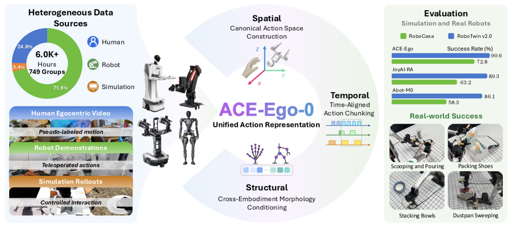
ACE-Ego-0: Unifying Egocentric Human and Robotic Data for VLA Pretraining
Vision-Language-Action models scale with embodied data, but teleoperated robot trajectories are expensive. Egocentric human video is abundant and depicts the same manipulation behaviors a robot must learn, yet four mismatches block joint training: action spaces (hand vs. end-effector), embodiment kinematics, control frequencies, and label fidelity (regressed pseudo-actions vs. sensor-logged ground truth). ACE-Ego-0 proposes a single VLA pretraining recipe that absorbs all of these sources by (i) projecting actions into a shared camera-frame interface, (ii) conditioning on morphology tokens, and (iii) downweighting noisy human supervision via an auxiliary head.
Unified action representation
The first contribution is a canonical action space that removes platform-specific coordinate conventions. All end-effector poses are expressed in the head-camera frame using the calibrated extrinsic R_{\mathrm{cam}\leftarrow s}, t_{\mathrm{cam}\leftarrow s}:
p_{\mathrm{cam}} = R_{\mathrm{cam}\leftarrow s}\, p_s + t_{\mathrm{cam}\leftarrow s}, \qquad R_{\mathrm{cam},ee} = R_{\mathrm{cam}\leftarrow s}\, R_{s,ee}.
Orientations use the continuous 6D parameterization of Zhou et al., with gripper commands and per-arm activity flags concatenated into a unified bimanual action vector. Because actions live in the same frame as the visual observations, the policy never has to learn world-to-camera transforms, and a new embodiment is integrated by swapping a single extrinsic plus its URDF-derived morphology token. At deployment the inverse transform recovers the execution frame:
\hat{p}_s = R_{\mathrm{cam}\leftarrow s}^{\top}(\hat{p}_{\mathrm{cam}} - t_{\mathrm{cam}\leftarrow s}), \qquad \hat{R}_{s,ee} = R_{\mathrm{cam}\leftarrow s}^{\top}\hat{R}_{\mathrm{cam},ee},
with the 6D rotation reconstructed via Gram–Schmidt before inversion.
Structural heterogeneity (humanoid AgiBot G1, single-arm wheeled Galaxea R1Lite, mobile-bimanual Galbot, and a “human surrogate” embodiment) is handled by morphology tokens derived from each source’s URDF, fed to the action expert alongside vision-language features. Temporal heterogeneity (10–30 Hz across platforms) is resolved with time-aligned action chunking so that a chunk corresponds to a fixed real-time horizon rather than a fixed step count.
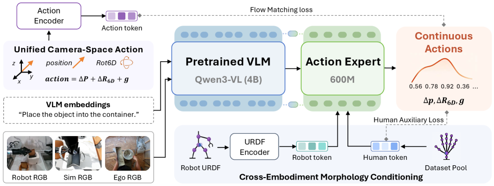
Reliability-aware training
Robot and simulation samples carry sensor-grounded labels and supervise the primary action expert directly. Human pseudo-actions, regressed from monocular video, are noisier in scale, contact, and occluded segments. ACE-Ego-0 routes them to an auxiliary loss head that shares the backbone but does not corrupt the primary expert’s parameters with high-variance gradients. The auxiliary objective concentrates supervision on segments flagged as reliable by the data pipeline, so human videos contribute representational priors (object affordances, motion priors, language grounding) while the action distribution at deployment remains anchored to robot demonstrations.
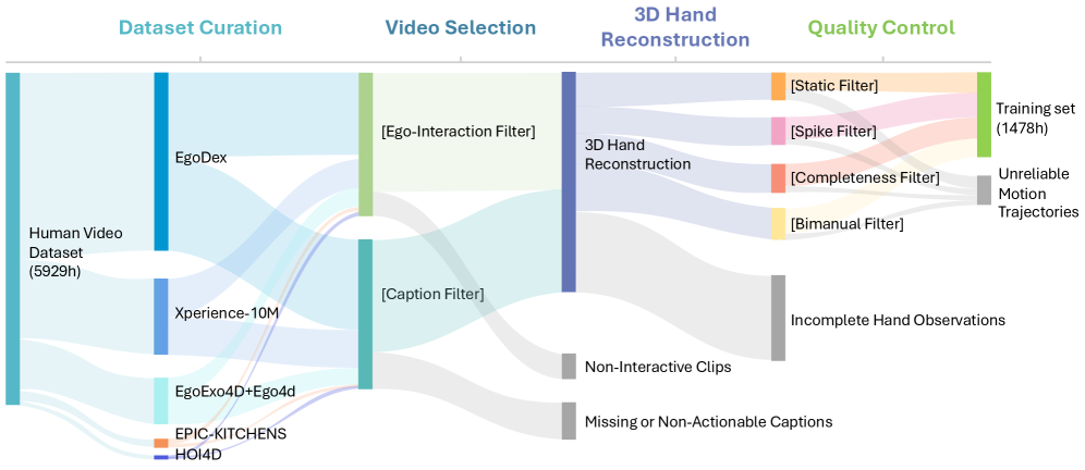
Data pipeline
The pretraining pool exceeds 6.0K hours and combines AgiBot Alpha/Beta demonstrations, Galaxea R1Lite data, AgiBot DigitalWorld and RoboCasa Tabletop simulation (24 tasks × 1,000 episodes on the GR1 humanoid), and 1,800+ hours of self-collected Galbot data. The egocentric branch contributes 1,478 hours of pseudo-action-labeled manipulation video extracted by a multi-stage pipeline: video selection, monocular motion reconstruction to recover wrist trajectories and hand poses, then multi-stage quality control to discard occlusion-heavy and non-manipulation segments before mapping the recovered hand pose into the bimanual action schema.
Experiments
Evaluation spans two simulation suites and one physical platform: RoboCasa GR1 TableTop (24 humanoid tabletop tasks), RoboTwin 2.0 (50 bimanual tasks with strong domain randomization), and an ARX bimanual real robot with six manipulation tasks. Baselines on RoboCasa include GR00T-N1.6, Qwen3PI, FLARE, ABot-M0, JoyAI-RA, and DIAL; on RoboTwin 2.0 the comparisons are against \pi_{0.5}, Motus, LingBot-VLA, ABot-M0, JoyAI-RA, and Hy-VLA. Real-robot comparisons use fine-tuned \pi_{0.5} and GR00T-N1.7. All evaluations are multi-task and report success rate. The provided sections describe the protocol but do not enumerate the headline numbers in the excerpt available; per-task tables (including \pi_0) are deferred to Appendix C.5.
Limitations and open questions
The framework leans on accurate camera extrinsics for both training-time canonicalization and deployment-time inversion; miscalibration directly biases the action space. Pseudo-action quality from monocular reconstruction remains the dominant noise source, and the reliability-aware auxiliary loss mitigates rather than removes it — there is no explicit uncertainty estimate fed into the loss weighting beyond pipeline-level filtering. Morphology tokens encode kinematics but not dynamics or actuator limits, so transfer to embodiments with very different control bandwidth may still require fine-tuning. Finally, head-camera-frame actions assume a stable, well-defined head camera, which is natural for humanoids and egocentric video but awkward for fixed third-person setups.
Why this matters
ACE-Ego-0 shows that the heterogeneity blocking joint human-video and robot pretraining is largely a representation problem: camera-space actions plus morphology tokens plus time-aligned chunking yield a single interface that consumes 1,478 hours of human video alongside ~4.5K hours of multi-embodiment robot and simulation data. If the recipe holds up under the appendix numbers, it provides a concrete template for scaling VLAs with non-teleoperated supervision.
Source: https://arxiv.org/abs/2606.17200
GameCraft-Bench: Can Agents Build Playable Games End-to-End in a Real Game Engine?
Problem and motivation
Most coding-agent benchmarks evaluate isolated functions, repository patches, or unit-test pass rates. Game generation breaks this mold: a “correct” output is not a passing test but a launchable artifact whose runtime behavior — scene graph, scripts, asset bindings, input handling, rendering, and gameplay loop — jointly realizes a natural-language design intent. The authors formalize end-to-end game generation as
x=(s,\mathcal{E})\ \longmapsto\ y=G,
where s is the spec (rules, mechanics, goals, presentation), \mathcal{E} is the development+runtime environment, and G is the produced game artifact, judged by observable player–game interaction. They argue any benchmark for this setting must satisfy three desiderata: Engine Grounding (agents must operate inside a real engine, not a sandbox), Artifact Completeness (produce a launchable project, not snippets), and Interactive Verification (score by replayed interactions, not static code inspection).
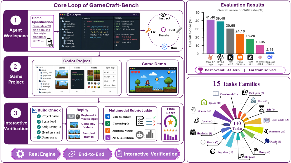
Benchmark construction
GameCraft-Bench instantiates the mapping in Godot. Each task is \tau=(s,\mathcal{E},\rho), where the rubric \rho is hidden from the agent. The environment is decomposed as \mathcal{E}=(\mathcal{R},\mathcal{W},\mathcal{A},\mathcal{C}): Godot runtime/toolchain \mathcal{R}, editable workspace \mathcal{W}, shared resource interface \mathcal{A}, and submission contract \mathcal{C}. The agent must return y=(G,\Pi), a complete Godot project plus replayable interaction traces \Pi=\{\pi_i\}_{i=1}^n. The verifier launches G in \mathcal{R}, executes
O=\mathrm{Replay}_{\mathcal{R}}(G,\Pi),
and feeds the resulting gameplay videos and sampled frames to a rubric-guided multimodal judge. Crucially, traces are evidence for evaluation, not part of the artifact — this separates “does the game work” from “did the agent script its own demo correctly.” The suite contains 140 tasks across 15 game families (platformers, shooters, puzzles, strategy skirmishes, etc.).
The rubric scores four axes: Mechanics (do core gameplay rules work), Depth (progression, state, secondary systems), Visuals (rendering correctness, UI legibility), and Art (stylistic coherence with spec).
Results
Seven frontier coding-agent configurations were run on all 140 tasks: Claude Code with Opus-4.7-high and MiMo-V2.5-Pro; Codex with GPT-5.5-high and DeepSeek-V4-Pro; Kimi Code with Kimi-K2.6; Code Buddy with GLM-5.1 and MiniMax-M2.7.
| Harness | Model | Overall | Mechanics | Depth | Visuals | Art |
|---|---|---|---|---|---|---|
| Claude Code | Opus-4.7 high | 41.46 | 55.34 | 39.48 | 42.78 | 36.86 |
| Codex | GPT-5.5 high | 39.49 | 54.36 | 38.61 | 41.84 | 32.94 |
| Kimi Code | Kimi-K2.6 | 30.65 | 39.76 | 28.07 | 33.66 | 27.99 |
| Claude Code | MiMo-V2.5-Pro | 24.10 | 32.33 | 22.59 | 27.45 | 20.65 |
| Code Buddy | GLM-5.1 | 18.29 | 25.23 | 17.80 | 21.14 | 14.59 |
| Code Buddy | MiniMax-M2.7 | 10.95 | 14.27 | 9.92 | 14.92 | 8.85 |
| Codex | DeepSeek-V4-Pro | 2.15 | 2.25 | 1.69 | 1.97 | 2.63 |
The best agent reaches only 41.46% overall; six of seven configurations score below 40%, and DeepSeek-V4-Pro under Codex collapses to 2.15% — likely a launchability/contract-compliance failure rather than a pure capability gap. Across all agents, Mechanics scores exceed Art scores, suggesting agents can implement recognizable gameplay loops more reliably than they can produce visually coherent presentations. The Depth axis lags Mechanics by 10–16 points for the top agents, indicating that secondary systems (progression, persistent state, balanced difficulty) are systematically under-implemented.
Diagnostic finding: rendered feedback as a debug signal
A standout analysis examines whether agents close the loop using rendered gameplay. Many failures (camera framing, unreadable HUD, broken layouts, demos that never trigger the intended mechanic) are invisible from source and stdout. The authors instrument screenshot-helper invocations across runs:
- Kimi-K2.6: 2,998 rendered-screen inspections over 140 tasks (mean 21.41, median 19); only 4 tasks used zero screenshots.
- Opus-4.7: 1,952 inspections (13.94 per task).
- GPT-5.5: 268 inspections (1.91 per task).
In a Strategy-Skirmish case, Kimi iteratively re-rendered the scene to detect misaligned unit placement and missing selection highlights, then patched the grid and turn-indicator. The pattern reframes game generation as perception-guided iteration rather than one-shot synthesis. Notably, GPT-5.5 achieves near-top overall scores while using screenshots ~10× less than Kimi or Opus, suggesting the relationship between visual debugging and final score is not monotonic — model priors over engine APIs likely substitute for visual verification up to a point.
Limitations and open questions
The benchmark is Godot-only; generalization to Unity/Unreal — with much larger surface APIs and asset pipelines — is unverified. Rubric-guided multimodal judging inherits the failure modes of the judge model; the paper does not report inter-judge agreement or human correlation. The submission contract requires agents to produce their own replay traces, which conflates gameplay correctness with the agent’s competence at scripting demonstrations of its own game. Finally, the DeepSeek-V4-Pro 2.15% outlier hints that contract/launchability failures dominate over capability differences for some configurations, which deserves a separate diagnostic axis (e.g., decoupled launchability vs. rubric scores).
Why this matters
GameCraft-Bench operationalizes a class of agent task that is genuinely end-to-end: success requires that runtime behavior in a real engine matches an open-ended specification, not that code passes tests. The 41.46% ceiling and the screenshot-usage analysis together suggest current coding agents are bottlenecked less by code synthesis than by closed-loop perception of their own artifacts.
Source: https://arxiv.org/abs/2606.17861
Hacker News Signals
Qwen-Robot Suite: A Foundation Model Suite for Physical World Intelligence
Alibaba’s Qwen team released a suite of models targeting robotics and embodied AI. The suite comprises several components: Qwen-VLo for vision-language-action, a unified multimodal model that ingests RGB observations and language instructions and outputs low-level motor commands; a world model component for predicting future states given actions; and tooling for sim-to-real transfer. The architecture extends Qwen2.5-VL with action-head layers that map latent representations to joint-space trajectories, trained on a mix of robot demonstration data and web-scale vision-language corpora. The approach follows the trend of treating manipulation policy learning as a sequence modeling problem, where action tokens are predicted autoregressively or via diffusion heads on top of a frozen or fine-tuned VLM backbone. Key claims include cross-embodiment generalization — one checkpoint deployed across multiple robot morphologies without architecture changes — and improved spatial reasoning via 3D-aware visual encoders. The blog is light on specific benchmark numbers (no table of task success rates), which limits independent evaluation. What matters practically: the models are released as open weights, making this directly usable for lab robotics stacks without the API dependency of RT-2 or Octo alternatives. Open questions remain around contact-rich manipulation, latency for real-time control loops (VLM inference at >100ms is a hard constraint for many tasks), and the quality and licensing of the demonstration data used for fine-tuning.
Source: https://qwen.ai/blog?id=qwen-robotsuite
How Memory Safety CVEs Differ Between Rust and C/C++
Jakub Beranek’s post performs a careful taxonomy of memory safety CVEs across Rust and C/C++ codebases, drawing on NVD data and case studies. The core argument is not simply “Rust has fewer memory safety bugs” but that the character of remaining bugs differs structurally. In C/C++, memory safety CVEs are predominantly spatial (buffer overflows, OOB reads/writes) and temporal (use-after-free, double-free) violations that arise from manual memory management. In Rust, memory safety CVEs cluster in a different region: unsafe blocks that contain incorrect invariant assertions, FFI boundary errors where raw pointers cross language boundaries without proper lifetime annotation, and integer overflow/truncation paths that feed into allocation sizes. The post identifies that Rust’s CVEs tend to require more application-specific context to trigger — they are not exploitable via generic heap spray techniques in the same way classic C bugs are. A second distinction: Rust’s type system pushes certain classes of concurrency bugs (data races) to near-zero, but logic errors in unsafe that corrupt state can still manifest as memory unsafety. The quantitative observation is that Rust codebases in production show CVE counts roughly proportional to the amount of unsafe surface, which tracks with what the ownership model actually guarantees. The post is appropriately cautious: it does not claim Rust eliminates memory safety vulnerabilities, only that it shifts the distribution toward bugs that are harder to exploit generically and often require auditing a smaller, explicitly marked code surface.
Source: https://kobzol.github.io/rust/2026/06/15/how-memory-safety-cves-differ-between-rust-and-c-cpp.html
Show HN: High-Res Neural Cellular Automata
This project extends the Neural Cellular Automata (NCA) framework — originally from Mordvintsev et al.’s “Growing Neural Cellular Automata” (2020) — to higher spatial resolutions. Standard NCAs operate on small grids (64x64 or 128x128) due to quadratic memory growth and instability at scale. The implementation addresses this by: (1) tiling the grid and running local update steps on patches with shared weights, reducing memory footprint; (2) using a gradient clipping and normalization scheme to stabilize training at higher resolutions where small perturbations propagate and amplify; (3) applying a perception kernel (Sobel filters for gradient estimation) that remains fixed regardless of resolution. The update rule follows the standard form: each cell’s state s_t is updated as s_{t+1} = s_t + f_\theta(P(s_t)) where P is the perception operator and f_\theta is a small MLP. The interest here is both aesthetic and technical — NCAs at high resolution reveal texture-level detail impossible at low res, and the tiling approach is a practical technique applicable to other grid-based learned dynamical systems. The live demo runs inference in-browser via WebGL/WASM, demonstrating that the per-cell compute budget is small enough for real-time execution. Limitations: the tiling introduces boundary artifacts at patch seams that require blending heuristics; training convergence remains slow relative to low-res variants; and target patterns must be carefully designed to remain stable under the update dynamics.
Source: https://cells2pixels.github.io/
Show HN: cuTile Rust: Safe, Data-Race-Free GPU Kernels in Rust
NVIDIA’s nvlabs released cuTile-rs, a Rust abstraction layer over their cuTile C++ tiling library for GPU kernel programming. The core contribution is a type-system encoding of GPU memory hierarchy that makes data races between threads within a cooperative thread array (CTA) a compile-time error. The mechanism uses Rust’s ownership and lifetime system: shared memory tiles are represented as typed resources with exclusive or shared borrow semantics, and the library’s barrier abstractions tie resource release to synchronization points, so a tile cannot be read before the corresponding __syncthreads() equivalent completes. At the PTX/SASS level, the generated code is equivalent to hand-written CUDA — the safety guarantees are purely in the Rust type layer with zero runtime overhead. The library targets Hopper and Blackwell architectures and exposes warpgroup-level matrix multiply-accumulate (WGMMA) instructions through safe wrappers. This matters because warpgroup programming is notoriously difficult: incorrect ordering of async copy operations and mma instructions with respect to barriers is a common source of silent correctness bugs that only manifest as numerical errors at scale. Limitations noted: the current API surface is narrow (dense matmul and attention-like patterns are well-supported; sparse or irregular access patterns require dropping into unsafe); Rust GPU toolchains remain immature relative to CUDA C (rustc-gpu/nvptx64 target has known codegen limitations); and the dependency on cuTile means portability to AMD/Intel GPUs is not addressed.
Source: https://github.com/nvlabs/cutile-rs
GLM-5.2 Is the New Leading Open-Weights Model on Artificial Analysis
Zhipu AI’s GLM-5.2 tops the Artificial Analysis Intelligence Index for open-weights models, a composite benchmark aggregating MMLU, MATH, HumanEval, and reasoning tasks with latency-normalized scoring. The model is a MoE architecture — specific expert counts are not publicly disclosed — available in a 32B active-parameter configuration. On the Artificial Analysis leaderboard it scores above Qwen2.5-72B and Llama-3.3-70B on the intelligence index while maintaining competitive tokens-per-second throughput on A100 hardware. The index methodology weights quality tasks at 70% and penalizes latency, so models that are fast-but-dumb or smart-but-slow are ranked lower than the headline accuracy numbers suggest. GLM-5.2 shows particular strength on Chinese-language tasks (expected given Zhipu’s training data composition) and on code generation, with reported HumanEval pass@1 in the mid-80s. Caveats: the Artificial Analysis index is a single aggregator’s composite metric, not a community-consensus benchmark; the model weights are available but the training data and RLHF procedure are not documented in a technical report. The HN discussion centers on whether leaderboard-optimized models represent genuine capability gains or benchmark saturation, and on the practical question of whether a 32B MoE fits in a cost-effective self-hosted configuration (rough answer: yes, on 2x A100 80GB with quantization).
Can Europe Train a Frontier AI Model on the Compute It Owns?
The euromesh repository is a structured analysis of European sovereign GPU compute capacity, aggregated from public procurement records, national AI initiative announcements, and supercomputing center inventories. The methodology: enumerate known H100/A100 clusters across GENCI (France), CINECA (Italy), SURF (Netherlands), BSC (Spain), and others; estimate usable FLOPs accounting for interconnect topology (many European clusters use InfiniBand HDR rather than NVLink, limiting tight coupling needed for large-model training); and compute whether the aggregate is sufficient to train a GPT-4-class model within a reasonable time horizon. The back-of-envelope math is sobering: European sovereign compute is estimated at roughly 50,000-80,000 H100-equivalents total, fragmented across 15+ institutions with no unified scheduling layer. Training a 500B-parameter dense model requires approximately 10^{25} FLOPs; at 50% MFU across the available cluster that implies multi-month runs with network latency between sites making pipeline parallelism across institutions essentially infeasible with current tooling. The repo points to network bandwidth between data centers (10-100 Gbps vs. 3.2 Tbps within an NVLink domain) as the binding constraint, not raw FLOP count. The discussion correctly identifies that EuroHPC’s upcoming systems (JUPITER, targeting 1 exaFLOP) change the arithmetic if scheduling policy allows long-running LLM jobs rather than the traditional short-allocation HPC model.
Source: https://github.com/sammysltd/euromesh
SubQ 1.1 Small: Technical Report
SubQ 1.1 Small is a compact language model targeting sub-1B parameter deployment, with a technical report covering architecture decisions and benchmark results. The model uses a standard decoder-only transformer with several modifications for efficiency: grouped-query attention (GQA) with a low group count to reduce KV cache size, SwiGLU activations, and a vocabulary distilled from a larger tokenizer to reduce embedding table size. Training uses a two-stage recipe: large-scale pre-training on a deduplicated web corpus followed by instruction fine-tuning with DPO. The reported benchmark numbers on tasks like HellaSwag, ARC-Easy, and Winogrande are competitive within the sub-1B tier (SmolLM2, Qwen2.5-0.5B range), though the report is transparent that the model does not exceed significantly larger models on reasoning-heavy tasks. The more interesting technical content concerns quantization behavior: the authors report that 4-bit GPTQ quantization degrades accuracy by less than 1.5% on aggregate benchmarks, attributed to the relatively uniform weight magnitude distribution from their training recipe. On-device inference targets include browser via ONNX/WebAssembly and microcontroller deployment via GGUF at int4. The report is honest about the primary use case being retrieval augmentation and classification tasks rather than open-ended generation, where latency constraints make sub-1B models practical and larger models are overkill.
Source: https://subq.ai/subq-1-1-small-technical-report
Ask HN: Has Anyone Replaced Claude/GPT with a Local Model for Daily Coding?
The thread generated 539 comments with a strong technical signal-to-noise ratio. The consensus across experienced practitioners: local models are viable for autocomplete and single-file edits using models in the 7B-32B range (Qwen2.5-Coder-32B and DeepSeek-Coder-V2-Lite cited most frequently), but fall short for multi-file refactoring and architectural reasoning tasks where context window management and instruction-following quality at the 100k+ token range still favor frontier APIs. Hardware requirements discussed: a 32B model at Q4_K_M quantization fits in 24GB VRAM (single RTX 4090 or 3090) and delivers 20-40 tok/s, which is acceptable for interactive use. Ollama and llama.cpp are the dominant serving stacks; several commenters report using Continue.dev or Aider as the editor integration layer. The latency-quality tradeoff is the central tension: local inference at 20 tok/s feels sluggish compared to Claude’s streaming at 80+ tok/s, particularly for long completions. A recurring observation is that the types of tasks matter more than aggregate benchmark scores — local models handle boilerplate, test generation, and regex construction well, while complex debugging across a large codebase still shows quality gaps. Cost calculus: at heavy API usage (~$50-100/month), the payback period on a 3090 is 6-12 months, but the privacy argument (no code leaving the machine) independently motivates the switch for many respondents working on proprietary codebases.
Noteworthy New Repositories
VibeBench/VibeSearchBench
A rigorous benchmark targeting conversational information-retrieval agents under realistic adversarial conditions. The 200 tasks are deliberately long-horizon: each starts with an intentionally vague query and unfolds through persona-driven progressive disclosure, meaning the agent must ask clarifying questions and update its retrieval strategy across multiple turns. This design stress-tests capabilities that single-turn benchmarks miss entirely — handling ambiguity, proactive information seeking, and multi-hop synthesis.
Evaluation avoids the schema-lock problem common in QA benchmarks: answers are represented as knowledge graphs and scored with triplet-level F1, so partial credit is structurally meaningful and there is no dependency on a fixed answer schema. The “verifiable” framing means each triplet can be independently checked against a ground-truth graph, keeping human annotation costs tractable at scale.
The benchmark is positioned as a direct counter to vibe-based agent evaluations where impressive demos mask shallow retrieval. For researchers building RAG pipelines, tool-augmented LLMs, or multi-turn dialogue systems, this provides a principled, hard test set. The 1000+ star count within days of release suggests practitioners have been waiting for exactly this kind of structured, adversarial, multi-turn retrieval benchmark.
Source: https://github.com/VibeBench/VibeSearchBench
CodeBendKit/codeseek
A Rust CLI that provides code-intelligence primitives designed specifically for consumption by AI coding agents rather than human IDEs. The core pipeline builds call graphs across seven languages (leveraging tree-sitter or similar AST tooling) and constructs hybrid search indexes combining dense embeddings, sparse BM25-style inverted indexes, and Reciprocal Rank Fusion (RRF) for score merging, with an optional reranker stage on top. This stack is the same retrieval architecture used in production semantic search systems, applied here to repository-scale code navigation.
The native output format is Model Context Protocol (MCP) tools, allowing Claude Code and Codex CLI to invoke call-graph traversal and hybrid code search directly as structured tool calls rather than shelling out to grep. Shipping as compiled Rust means sub-second index queries even on large codebases, which matters when an agent is making many sequential retrieval calls per task.
The project is practically useful for anyone instrumenting an agentic coding workflow that needs structured codebase understanding beyond naive file concatenation — particularly for refactoring, dependency tracing, and cross-file symbol resolution.
Source: https://github.com/CodeBendKit/codeseek
perplexityai/bumblebee
A read-only scanner from Perplexity AI that enumerates on-disk metadata for installed packages, browser/editor extensions, and developer tools, then cross-references that inventory against known software supply-chain compromise databases. The read-only constraint is architecturally deliberate: the tool never modifies state, making it safe to run in CI or on production build machines without risk of side effects.
The threat model it addresses is concrete — dependency confusion attacks, typosquatted packages, and compromised extensions have become a significant attack surface in developer environments (XZ utils, the npm socket.io-parser incident, malicious VS Code extensions). Bumblebee provides a systematic audit rather than relying on developers to manually track advisories.
Built to be a developer endpoint scanner rather than a full SAST tool, it focuses narrowly on supply-chain exposure: what is installed, what version, and does it appear in known-bad lists. The narrow scope keeps false-positive rates low. At 4400+ stars on day one, demand for this kind of targeted supply-chain visibility in developer tooling is clearly high.
Source: https://github.com/perplexityai/bumblebee
omnigent-ai/omnigent
A meta-harness providing a unified abstraction layer over heterogeneous AI coding agents — Claude Code, OpenAI Codex, and user-defined agents can be addressed through a common interface, with runtime switching or parallel combination without rewriting task orchestration logic. The key architectural additions beyond simple routing are policy enforcement and sandboxing: operators can specify constraints on what actions agents are permitted to take, enforced at the harness level rather than relying on each agent’s internal guardrails.
The collaborative multi-user session model is technically interesting — multiple clients can observe and interact with the same live agent session in real time, which enables human oversight workflows (one person writing, another auditing) and paired agent collaboration patterns.
For organizations running multiple agent types across different tasks, the value is operational: a single integration point reduces the surface area of agent-specific plumbing. The policy layer addresses a real gap in current agent deployments where per-agent sandboxing is either absent or requires bespoke implementation. Early traction (3200+ stars) suggests teams are actively looking for this kind of multi-agent governance layer.
Source: https://github.com/omnigent-ai/omnigent
amElnagdy/guard-skills
A collection of quality-gate “skills” — structured checks that can be inserted into AI coding agent pipelines to catch characteristic failure modes in LLM-generated code, tests, and documentation. The framing as skills rather than linters is deliberate: these are designed to be invoked by agents themselves as self-evaluation steps, not just run post-hoc by humans.
The failure modes targeted are specifically those that trip up AI code generators: plausible-but-wrong test assertions, hallucinated API signatures, documentation that drifts from implementation, and shallow test coverage that passes surface checks while missing edge cases. Static linters catch syntactic and type errors; these guards target semantic correctness at the agent-output layer.
The practical deployment pattern is as a step in an agentic coding loop — generate, guard, revise — rather than as a one-shot post-processor. This aligns with how production agent harnesses like Claude Code and Codex workflows are increasingly structured. Useful for teams integrating AI coding into CI who want machine-checkable quality bars beyond compilation and existing lint rules.
Source: https://github.com/amElnagdy/guard-skills
packyme/privacy-filter
A Go service acting as a transparent proxy between application code and LLM APIs, performing millisecond-latency PII and secret detection/redaction before requests leave the network perimeter. The performance claim — millisecond latency — implies rule-based and pattern-matching approaches (regex, NER with compiled models, or similar) rather than a second LLM call, which would add hundreds of milliseconds and significant cost.
The threat model is straightforward: developers sending prompts that inadvertently include API keys, credentials, names, email addresses, or other regulated data into cloud LLM endpoints. A gateway architecture means no changes to application code are required — requests are intercepted and scrubbed at the network layer.
Implemented in Go for concurrency efficiency and low GC overhead, making it suitable as a sidecar or in-process library in high-throughput services. The production deployment claim by PackyCode provides some evidence of real-world validation. For teams subject to GDPR, HIPAA, or SOC 2 requirements who are integrating LLM calls into production services, this addresses a concrete compliance gap that most LLM SDK integrations ignore entirely.
Source: https://github.com/packyme/privacy-filter
1ove9/antenna-forge
An inverse antenna design tool that uses AI-driven optimization with real electromagnetic simulation in the loop — specifically NEC2 (Method of Moments, widely used for wire antennas) and openEMS (FDTD-based full-wave simulation). Inverse design here means specifying target RF performance characteristics (gain pattern, impedance, bandwidth) and having the optimizer search antenna geometry space to meet them, rather than the forward problem of simulating a known geometry.
The dual-simulator approach is notable: NEC2 is fast and suitable for wire/monopole geometries, while openEMS handles more complex 3D structures including substrate effects, making the tool useful across a broader antenna design space. The AI component presumably drives the optimization loop — likely gradient-free methods (evolutionary algorithms, Bayesian optimization) since EM simulators are not differentiable.
The in-browser playground reduces the barrier to entry significantly for RF engineers who want to experiment without a local NEC2/openEMS installation. Antenna design remains a domain where physical simulation is non-negotiable for reliable results, so keeping real simulators in the loop rather than using a surrogate-only approach is the right engineering choice.
Source: https://github.com/1ove9/antenna-forge
ATOM00blue/machine-learning-library
A curated, structured corpus of 923 ML learning resources: 391 arXiv papers, 474 lecture materials (Stanford, MIT, Karpathy, fast.ai), and 58 explainer articles, all normalized to Markdown with preserved provenance metadata. The normalization step is the substantive engineering here — converting PDFs, notebooks, and HTML lecture notes to clean Markdown with consistent frontmatter enables programmatic use cases that raw PDFs block.
Three concrete use cases are supported by the format choices: (1) human study in Obsidian, where the graph view over topic-organized notes provides navigable structure; (2) RAG corpora, where clean Markdown with metadata enables reliable chunking and retrieval; (3) fine-tuning datasets, where provenance tracking is necessary for dataset cards and attribution. The topic organization imposes a taxonomy that aids retrieval quality in both human and automated contexts.
The value over a raw arXiv scrape is curation and normalization: someone has already done the selection (filtering for pedagogical quality rather than just recency) and the format conversion (removing LaTeX rendering artifacts, fixing encoding issues). For researchers bootstrapping a domain-specific RAG system or synthetic training data pipeline on ML content, this is a substantially lower-effort starting point than building the corpus from scratch.
Source: https://github.com/ATOM00blue/machine-learning-library