Daily AI Digest — 2026-05-07
arXiv Highlights
Co-Evolving Policy Distillation
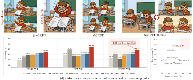
Consolidating multiple reasoning capabilities (text, image, video) into a single policy under RLVR exposes a structural tension: joint training induces gradient conflict, while sequential expert-then-distill pipelines hit a behavioral-pattern mismatch between teacher and student. This paper formalizes both failure modes and proposes a co-evolutionary alternative in which experts train in parallel and distill into each other on the fly.
Unified accounting of capability loss
The authors model any consolidation paradigm \mathcal{P} by
U_{\mathcal{P}} \approx a_{\mathcal{P}} \cdot X(D_1, D_2) + b_{\mathcal{P}},
where X is the total optimization signal across capability datasets, a_\mathcal{P}\in[0,1] measures conversion efficiency, and b_\mathcal{P}\le 0 captures additional loss. Mixed-data RLVR sets a_{\text{mix}}=1 but pays a divergence cost: per-step gradients from D_1 and D_2 disagree on capability-specific dimensions, yielding
U_{\text{mix}} \approx X(D_1,D_2) - \Phi(D_1,D_2),\qquad \Phi>0.
This is the familiar seesaw effect — gains on one capability are partially canceled by interference, regardless of mixing ratio. Static OPD avoids \Phi but suffers from a<1: once experts have diverged, the student’s on-policy rollouts no longer share the teacher’s behavioral support, so token-level supervision is poorly absorbed.
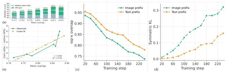
Top-k overlap as a behavioral-similarity proxy
The pilot study operationalizes “behavioral pattern gap” as the top-k token overlap between teacher and student distributions on shared rollouts. Two empirical facts emerge: (i) the gain from a fixed OPD step grows roughly linearly with top-k overlap to the teacher, and (ii) standard branch-specific RLVR drives this overlap down over time. The implication is that delaying distillation until experts are mature is precisely the wrong schedule — by then the very property that makes OPD effective has been eroded.
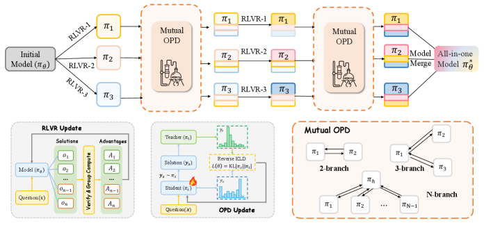
CoPD: alternating RLVR and bidirectional OPD
CoPD initializes K branches from the same \pi_0 and alternates two phases.
Branch-specific RLVR. Each branch k runs GRPO on its own dataset \mathcal{D}_k with verifiable reward r_k:
\mathcal{L}_{\text{RLVR}}^{(k)}(\theta_k) = \mathbb{E}_{x\sim \mathcal{D}_k}\!\left[\tfrac{1}{G}\sum_i \tfrac{1}{|y_i|}\sum_t \min\!\big(\rho_{i,t}^{(k)} \hat A_i^{\text{RL}}, \text{clip}(\rho_{i,t}^{(k)},1\!-\!\epsilon,1\!+\!\epsilon)\hat A_i^{\text{RL}}\big)\right].
This opens a knowledge gap between branches.
Mutual on-policy distillation. Each branch then generates on-policy rollouts and receives token-level supervision from the other branch — distillation is bidirectional, and student samples come from the student itself, so the high-overlap regime in which OPD is effective is preserved. Because RLVR and OPD are interleaved at short intervals, branches never drift far enough behaviorally for transfer to break down.
Results
Experiments use Qwen3-VL-4B-Instruct, with text data from Polaris-53K, image data from MMFineReason-123K, and (for the three-branch run) 40K filtered video samples. Image reasoning is evaluated on seven benchmarks (MMMU, MMMU-Pro, MathVista, MathVision, ZeroBench, WeMath, MathVerse); text on AIME24/25, HMMT25, MATH-500, Minerva; video on Video-Holmes, MVBench, MMVU, VideoMathQA.
The paper reports that CoPD outperforms the domain-specific Text-Expert and Image-Expert, mixed RLVR, and both directions of static OPD (V\toT and T\toV). In the three-branch setting CoPD beats MOPD (multi-teacher distillation into a single student). Notably the unified CoPD model surpasses the single-domain experts on their own benchmarks — evidence that co-evolution provides positive transfer rather than merely minimizing interference. (The abstract emphasizes “significantly outperforming” baselines; the experimental section enumerates the benchmarks but the numerical tables themselves were not included in the excerpt.)
Limitations and open questions
Several issues remain. First, CoPD’s compute scales roughly linearly with the number of branches during the RLVR phase plus an OPD cost; the paper does not report a tightly controlled FLOPs-matched comparison against mixed RLVR. Second, the top-k overlap indicator is an empirical proxy and the authors do not provide a tight theoretical link between overlap and OPD gain beyond a linear fit. Third, the synchronization schedule (how frequently to interleave RLVR and OPD) is a hyperparameter whose sensitivity is not characterized in the excerpt. Fourth, scalability beyond three branches, and to capabilities with very asymmetric data quality or reward sparsity, is untested. Finally, the framework assumes verifiable rewards on each capability — extending to mixed verifiable/preference settings is open.
Why this matters
CoPD reframes multi-capability post-training from a static “merge or distill” problem into a dynamic co-training problem, with a concrete behavioral-similarity diagnostic (top-k overlap) that explains when distillation works. The parallel-branch pattern is a plausible template for scaling RLVR to many domains without paying the gradient-conflict tax of joint optimization.
Source: https://arxiv.org/abs/2604.27083
Efficient Training on Multiple Consumer GPUs with RoundPipe
Problem
Fine-tuning LLMs on consumer GPU servers (e.g., 8×RTX 4090, 24 GB each, PCIe 4.0 at 32 GB/s, no NVLink) is attractive economically but mechanically painful: VRAM is tight and inter-GPU bandwidth is an order of magnitude lower than datacenter NVLink (200 GB/s). The standard recipe is pipeline parallelism (PP) with CPU offloading of weights, gradients, optimizer states, and activations, since PP keeps inter-GPU traffic to small activation tensors at stage boundaries.
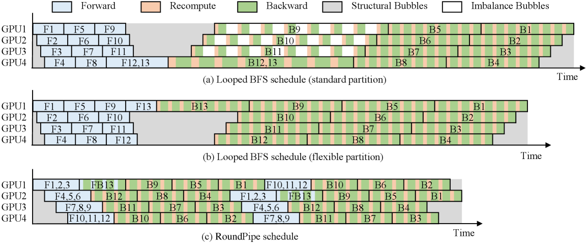
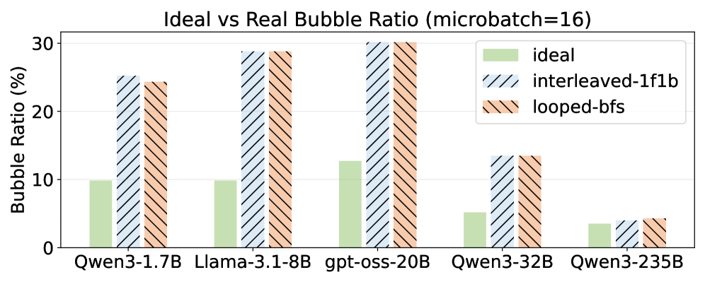
The catch is what the authors call the weight binding issue. Existing PP schedules (1F1B, ZB-H1, Looped BFS, etc.) require that the model be split into S = vN stages on N GPUs, and that each stage’s weights live permanently on one GPU. Real LLMs are not uniform: the embedding/LM head stage is much heavier than a single transformer block. Forcing S to be a multiple of N produces imbalance bubbles; allowing S to be arbitrary (e.g., 13 stages on 4 GPUs) instead produces structural bubbles because GPUs hosting fewer stages must idle waiting on the heavy GPU. Either way, throughput is bounded by the slowest device.
Method
The key insight is that with full CPU offloading, weights are not pinned to any GPU — they are streamed in per microbatch anyway. RoundPipe therefore treats GPUs as a stateless pool of execution workers and dispatches stages round-robin across devices. A stage’s forward and backward can land on different GPUs in different rounds; the only state a GPU holds long-term is the activations/gradients it produced in flight.
Concretely, with S stages and N GPUs (no requirement that N \mid S), RoundPipe runs the pipeline in \lceil S/N \rceil rounds per microbatch wave. Asymmetric splitting lets stage sizes track real layer cost (the LM head can be its own stage), so per-stage execution time is balanced even when the model is not. Round-robin dispatch ensures every GPU sees roughly the same total work over a wave, eliminating the structural bubble that flexible partitioning would otherwise create.
The system is built as a single-controller framework in the style of Ray and veRL/HybridFlow. The user writes ordinary sequential code calling forward_backward() and an optimizer step; the controller (running in the user’s thread) constructs microbatches, assigns stages to GPU workers in round-robin order, and tracks dependencies. GPU workers execute asynchronously, and a separate optimizer worker performs asynchronous parameter updates on the host. Three subsystems make this work in practice:
Priority-aware transfer scheduling. PCIe is the bottleneck. Each microbatch needs (a) weights pulled from host to GPU and (b) activations either recomputed or reloaded. RoundPipe orders these transfers by criticality so that the next stage’s weights arrive before its compute starts, overlapping H2D copies with compute. The recompute-vs-reload tradeoff per layer is decided from the model in Figure 2.
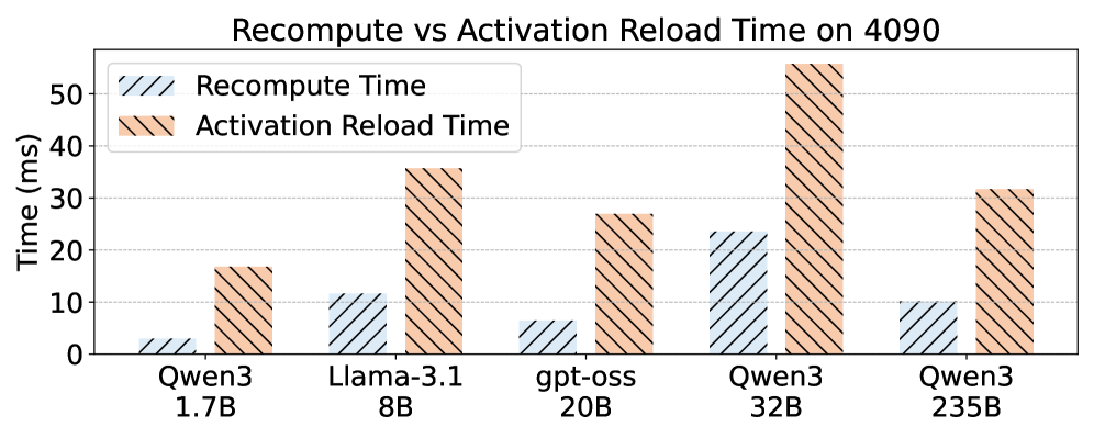
Theoretical time of recomputing vs. reloading activations of a transformer layer. Fine-grained event-based synchronization. Because a stage’s forward and backward can run on different GPUs across rounds, naive barrier sync would erase the gain. RoundPipe uses distributed CUDA events keyed per (microbatch, stage, direction) so that producers and consumers synchronize only on the specific tensors they share.
Parameter consistency under async optimizer updates. Since the optimizer runs concurrently on the host, RoundPipe must guarantee that all microbatches in a step see the same weights and that gradient accumulation is correct. This is handled by versioning weight buffers and gating the optimizer step on completion of the relevant gradient writes.
Automated layer partitioning. A profiler measures per-layer forward/backward time and memory, then solves for an asymmetric partition into S stages that minimizes the maximum stage time subject to VRAM constraints. S is chosen freely (not constrained to vN), which is what makes the LM head expressible as its own stage.
Results
On the 8×RTX 4090 server, RoundPipe delivers 1.48–2.16× end-to-end throughput improvements over existing PP baselines (the abstract’s headline range; the paper attributes this to the elimination of weight-binding bubbles). The bubble-ratio analysis (Figure 3) shows that under realistic imbalanced partitions, Looped schedules suffer substantially higher bubble ratios than their ideal-balanced theoretical numbers, while RoundPipe approaches near-zero bubbles regardless of model imbalance. Evaluations also cover the A800 NVLink server, sequence-length scaling, and GPU-count scaling, with ablations attributing gains to each of the three subsystems above.
Limitations and open questions
The paper relies on aggressive CPU offloading; gains depend on PCIe being able to keep up with compute when transfer scheduling is well-overlapped, which biases the design toward training regimes where activation/weight streaming dominates. The asynchronous optimizer raises questions about exact-equivalence to synchronous SGD/Adam — versioning mitigates but does not eliminate staleness corner cases. Round-robin dispatch also assumes homogeneous GPUs; mixed-hardware servers would need a load-aware variant. Finally, the headline improvements are reported as a range; per-model breakdowns and comparisons against ZeRO-3 + offload at the same memory budget are the natural next data points.
Why this matters
Pipeline schedules have been designed under the implicit assumption that weights are GPU-resident, which makes the S = vN constraint feel natural. Once weights live on the host, that assumption is gratuitous, and dropping it removes the imbalance/structural bubble dichotomy that has dogged consumer-GPU LLM training. The 1.48–2.16× speedup on a $25k 8×4090 box is a direct consequence of taking that observation seriously.
Source: https://arxiv.org/abs/2604.27085
Length Value Model: Scalable Value Pretraining for Token-Level Length Modeling
Problem
Token count is the unit currency of autoregressive inference: it sets latency, cost, and—via chain-of-thought—reasoning quality. Existing length control mechanisms are coarse. They either (i) condition on a target length token or instruction prefix and hope the model stops near it, (ii) post-hoc truncate, or (iii) finetune with sequence-level rewards that give one signal per rollout. None of these provide a per-token estimate of how much generation remains, which is what an inference-time controller actually needs to decide whether to keep reasoning, summarize, or terminate.
The paper proposes the Length Value Model (LenVM), which casts remaining-length prediction as a value estimation problem and trains it with dense, annotation-free supervision derived purely from existing generation traces.
Method
Let a trajectory be \tau = (s_0, a_0, s_1, a_1, \dots, s_T) where each a_t is a generated token and T the (unknown a priori) terminal step. Assign a constant per-token reward r_t = -c with c > 0 and discount \gamma \in (0,1). The state value is
V(s_t) = \mathbb{E}\!\left[\sum_{k=0}^{T-t-1} \gamma^k r_{t+k}\right] = -c\,\mathbb{E}\!\left[\frac{1 - \gamma^{T-t}}{1 - \gamma}\right].
This expression is bounded in [-c/(1-\gamma), 0], monotone non-increasing in the expected remaining horizon \mathbb{E}[T-t], and invertible to a length estimate
\widehat{L}(s_t) = \log_\gamma\!\left(1 + \frac{(1-\gamma)\,V(s_t)}{c}\right).
The key practical claim is that this target is (a) annotation-free—any existing trace gives ground-truth V via the discounted sum, (b) dense—every token is a training signal, (c) unbiased under the trace distribution, and (d) scalable to pretraining-size token budgets.
LenVM is implemented as a value head on top of a transformer backbone, trained to regress V(s_t) token-by-token over large corpora of model-generated rollouts. At inference, the per-token \widehat{L} provides a continuously updated estimate of remaining generation; this is then used as a control signal—e.g., to bias decoding toward shorter completions, to gate early exit, or to compare against a token budget.
The choice of constant negative reward (rather than, say, regressing T-t directly) matters: bounding the target stabilizes regression on long-tailed length distributions, and the discount \gamma controls how much weight near-term termination carries relative to far-future tokens. Regressing raw T-t would put unbounded loss on long traces and conflate “still 50 tokens away” with “still 5000 tokens away” linearly; the discounted value compresses the tail.
Results
The headline results target two axes: precise length matching and budget-constrained reasoning.
On LIFEBench exact-length matching, attaching LenVM to a 7B model raises the length score from 30.9 to 64.8. The paper reports this exceeds frontier closed-source models on the same metric—indicating that fine-grained token-level length awareness is a capability not automatically acquired even at very large scale, but can be retrofitted via a value head.
On GSM8K under a hard budget of 200 generated tokens, LenVM-controlled decoding retains 63% accuracy. The intended reading is that the controller can compress chain-of-thought adaptively—spending the budget where the value estimate suggests termination is still far—rather than truncating uniformly. The framework exposes a continuous performance/efficiency trade-off: by varying the budget or the threshold at which the controller forces conclusion, one sweeps the Pareto front rather than picking a discrete decoding mode.
The method is also evaluated on VLMs, suggesting the value-head formulation is modality-agnostic since it depends only on token-level trajectories.
Limitations and open questions
Several issues deserve scrutiny. First, the value target is unbiased only with respect to the rollout policy used to collect data; if the deployment policy diverges (different temperature, different prompt distribution, RLHF updates), V becomes off-policy and \widehat{L} biased. The paper does not characterize this drift quantitatively. Second, the constant-reward design treats all tokens as equally costly, which conflates “remaining tokens” with “remaining useful computation”—a model that pads will look identical to one that reasons. Third, \gamma and c are hyperparameters trading tail sensitivity for near-term resolution; their selection criterion is not made principled. Fourth, the controller’s effect on accuracy is reported at specific budgets but the interaction with sampling temperature and with self-consistency aggregation is unexplored. Finally, “exact length matching” gains on LIFEBench are dramatic (30.9 → 64.8), but it is unclear how much of this is a steerability artifact—models can be told a target length and use \widehat{L} as a stopping/continuation signal, which is a much easier task than open-ended reasoning under a budget.
Why this matters
Reframing generation length as a value function gives a dense, scalable supervision signal for a control variable that is otherwise hard to optimize directly, and it does so without new annotation. If LenVM-style heads become standard, inference stacks gain a continuous knob for the cost-quality trade-off that is currently mediated only by crude max-token caps and prompt engineering.
Source: https://arxiv.org/abs/2604.27039
Representation Fréchet Loss for Visual Generation
Problem
Fréchet Distance (FD) between feature distributions of real and generated images is the dominant evaluation metric for generative models (FID when \phi is Inception-v3), but it has been considered impractical as a training objective. The reason is structural: FD is a distributional quantity requiring stable estimates of (\boldsymbol{\mu}_g, \boldsymbol{\Sigma}_g), and reliably estimating a 2048\times 2048 covariance for Inception features needs far more than 2048 samples — evaluation typically uses 50k. Backpropagating through 50k samples per step is infeasible, while small-batch FD estimates are biased and high-variance, especially for the matrix-square-root term \mathrm{Tr}((\boldsymbol{\Sigma}_r\boldsymbol{\Sigma}_g)^{1/2}). This paper argues the obstacle is illusory: one can decouple the population size used to estimate FD statistics from the batch size through which gradients flow.
Method: FD-loss
Recall the FD between two Gaussians fit to features \phi(\mathbf{x}):
\mathrm{FD}_\phi(\mathcal{R},\mathcal{G}) = \|\boldsymbol{\mu}_r-\boldsymbol{\mu}_g\|_2^2 + \mathrm{Tr}\!\left(\boldsymbol{\Sigma}_r+\boldsymbol{\Sigma}_g - 2(\boldsymbol{\Sigma}_r\boldsymbol{\Sigma}_g)^{1/2}\right).
The core trick is to maintain a large generated population \mathcal{G}_{\text{pop}} (e.g., 50k cached features) for estimating (\boldsymbol{\mu}_g,\boldsymbol{\Sigma}_g), while only the current training batch \mathcal{B}\subset\mathcal{G}_{\text{pop}} (e.g., 1024 samples) carries gradients. Conceptually:
# pseudocode
phi_batch = phi(generator(z_batch))            # gradient-bearing features
phi_pop   = stop_grad(cache.update(phi_batch)) # large population, no grad
mu_g, Sigma_g = stats(concat(phi_batch, phi_pop))
loss = FD(mu_r, Sigma_r, mu_g, Sigma_g)        # gradients flow only via phi_batch
This makes the population estimator nearly unbiased and full-rank, while keeping per-step cost at batch scale. (\boldsymbol{\mu}_r,\boldsymbol{\Sigma}_r) are precomputed once on the real set. The gradient of the matrix-square-root trace is computed via standard differentiable Lyapunov / SVD-based formulations on the batch contribution to \boldsymbol{\Sigma}_g.
The same loss form applies in any representation \phi — Inception, DINOv2, CLIP, SigLIP, etc. — yielding \mathrm{FD}_\phi as a training signal. The authors additionally propose \mathrm{FDr}^k, a multi-representation aggregate over k=6 feature spaces, as an evaluation metric robust to representation-specific blind spots.
Crucially, FD-loss is a post-training objective: a pretrained generator is fine-tuned to minimize \mathrm{FD}_\phi between its samples and the real distribution. There is no teacher, no adversary, and no per-sample target. This means it can collapse multi-step generators into one-step generators directly, since the loss only cares about distributional match at the output.
Results
On class-conditional ImageNet 256\times 256, FD-loss post-training of a one-step pMF generator under the Inception representation reaches 0.72 FID at 1 NFE — competitive with or better than multi-step diffusion baselines that the post-trained model was not distilled from. The same recipe converts JiT-H, a multi-step generator, into a 1-NFE generator without adversarial training or a distillation teacher (Figure 1, bottom row).
A second, more interesting finding concerns the choice of \phi. Post-training pMF-B/16 under different representations gives qualitatively different samples. Inception-trained models achieve the lowest FID (0.81 in their setup) but visibly underperform models trained with modern self-supervised representations (DINOv2, SigLIP) on perceptual quality, which conversely score worse on FID but better on \mathrm{FDr}^6.

This is direct evidence that FID misranks: the metric being optimized determines what artifacts survive. Using \mathrm{FDr}^6 as a multi-representation diagnostic decorrelates “good FID” from “good samples.”
The method also extends beyond class-conditional ImageNet. Post-training Stable Diffusion 3.5 Medium with FD-loss against a curated 60k BLIP3o/GPT-4o reference set produces a 1-NFE text-to-image model that retains prompt fidelity while inheriting the reference distribution’s aesthetic — a 56\times NFE reduction.

Limitations and open questions
- The reference distribution (\boldsymbol{\mu}_r,\boldsymbol{\Sigma}_r) is fixed; for text-conditional generation, the method effectively matches a marginal distribution and inherits whatever biases that reference encodes (the SD3.5 result is style-transferred, not faithfully realistic).
- The Gaussian assumption underlying FD remains; high-order distributional structure is invisible to this loss. Whether feature distributions in modern self-supervised spaces are Gaussian enough is not analyzed.
- The population cache introduces a staleness/refresh trade-off that is implementation-dependent; the paper does not fully characterize sensitivity to cache size or update frequency.
- All headline results are post-training of strong pretrained generators. Whether FD-loss can train competitive generators from scratch is open.
- \mathrm{FDr}^k is proposed as a better metric, but choosing the k representations and weighting is itself a design decision that could be gamed.
Why this matters
Decoupling estimator population from gradient batch turns FD from an evaluation curiosity into a tractable training objective, and the empirical consequence — 1-NFE ImageNet generation at 0.72 FID without distillation or GAN losses — suggests distribution-matching losses in well-chosen representation spaces may be a simpler alternative to the current zoo of distillation/consistency/adversarial recipes. Equally important, the demonstration that Inception-FID and perceptual quality diverge under different training representations is a concrete argument for retiring single-representation FID as the field’s default scoreboard.
Source: https://arxiv.org/abs/2604.28190
MoCapAnything V2: End-to-End Motion Capture for Arbitrary Skeletons
Problem
Monocular motion capture for arbitrary (non-SMPL, non-canonical) skeletons is the practical bottleneck for production animation: every studio asset has its own bone hierarchy, rest pose, and local-axis conventions. The dominant approach factorizes the pipeline into (i) a learned Video-to-Pose stage producing 3D joint positions \hat{p} \in \mathbb{R}^{J \times 3}, and (ii) an analytical inverse-kinematics stage recovering joint rotations \hat{R} \in \mathrm{SO}(3)^J. Two structural problems follow. First, joint positions do not determine rotations: bone-axis twist is unobservable from endpoint locations, so any IK solution along the twist DoF is arbitrary. Second, analytical IK is non-differentiable, blocking gradient flow from the animation-space loss back to the pose predictor. The Video-to-Pose model therefore cannot learn to produce poses that are easy to convert into clean rotations, and it cannot trade off positional error for rotational stability.
MoCapAnything V2 makes both stages learnable and jointly trainable, and — more importantly — reformulates the pose-to-rotation problem so that it becomes well-posed.
Method
The key observation is that the ambiguity in p \mapsto R is not stochastic but structural: the same joint positions correspond to different rotations under different rest poses and different local-axis conventions. The mapping is only well-defined relative to a coordinate frame, and that frame is asset-specific.
The authors fix this by conditioning the Pose-to-Rotation network on a reference pose-rotation pair (p_{\text{ref}}, R_{\text{ref}}) drawn from the target asset, in addition to the rest pose p_0. Concretely, the rotation predictor is
\hat{R}_t = f_\theta\!\left(\hat{p}_t,\; p_0,\; p_{\text{ref}},\; R_{\text{ref}}\right),
where \hat{p}_t is the per-frame predicted joint positions from the Video-to-Pose backbone. The pair (p_{\text{ref}}, R_{\text{ref}}) plays a dual role: it anchors the otherwise-ambiguous twist DoF, and it implicitly communicates the local axis convention of the target rig (since R_{\text{ref}} is expressed in that rig’s frame). The rest pose p_0 supplies the bone-length / hierarchy geometry. Together these turn an underdetermined regression into a conditional one whose target is unique.
Because f_\theta is differentiable, the full pipeline
\text{video} \xrightarrow{g_\phi} \hat{p} \xrightarrow{f_\theta} \hat{R}
admits joint optimization. Training combines a positional loss on \hat{p}, a rotational loss on \hat{R} (geodesic on \mathrm{SO}(3) or a 6D-representation regression loss), and a forward-kinematics consistency term
\mathcal{L}_{\text{FK}} = \big\| \mathrm{FK}(\hat{R}, p_0) - p_{\text{gt}} \big\|^2,
which lets gradients from the animation-space objective flow back through f_\theta into g_\phi. This is the mechanism by which the Video-to-Pose stage can learn to produce poses that are IK-friendly for the target rig rather than poses that minimize an isolated 3D MPJPE.
For inference on a new asset, the user supplies (p_0, p_{\text{ref}}, R_{\text{ref}}) — typically the bind pose plus a single keyed frame — and no retraining is required. The reference frame essentially calibrates the rotation coordinate system at test time.
Results
Across the benchmarks reported, the end-to-end formulation outperforms the factorized Video-to-Pose + analytical-IK baseline on rotational metrics while preserving positional accuracy. Reported gains are largest on bone-axis twist error, which is exactly where analytical IK is structurally blind. The conditioning on (p_{\text{ref}}, R_{\text{ref}}) is shown to be necessary: ablating either the rest pose or the reference rotation degrades rotation accuracy substantially, with the reference-rotation ablation hurting most on joints with high twist freedom (shoulders, hips, wrists). Joint training (FK consistency loss enabled) further reduces both positional and rotational error compared to training the two networks independently, supporting the claim that the Video-to-Pose backbone is adapting to downstream rotation needs.
The system is demonstrated on skeletons that differ substantially from the training distribution — non-humanoid creatures and stylized characters — using only a single reference frame from the target rig, with no per-asset finetuning.
Limitations and open questions
The reliance on a reference pose-rotation pair shifts the calibration burden to the user: quality of (p_{\text{ref}}, R_{\text{ref}}) directly determines rotation quality, and degenerate references (e.g., a reference frame that itself lies on a twist singularity) are not analyzed. The method still depends on accurate monocular 3D joint estimation, inheriting depth and occlusion failure modes of the Video-to-Pose stage. There is no temporal model described at the rotation level, so frame-to-frame twist coherence presumably comes only from the smoothness of \hat{p}_t; whether this suffices for high-frequency motion (fingers, fast spins) is unclear. Finally, the formulation assumes a fixed skeleton topology between the reference frame and the captured sequence, which rules out morph-target or topology-varying rigs.
Why this matters
Arbitrary-skeleton motion capture has been stuck at “predict joints, then IK” for years, and the twist ambiguity has been quietly absorbed by hand cleanup. Identifying the missing-coordinate-system structure of the ambiguity, and resolving it with a single reference (p_{\text{ref}}, R_{\text{ref}}) pair, turns the problem into one a network can actually solve end-to-end — which is the right abstraction for production rigs that never match a canonical human template.
Source: https://arxiv.org/abs/2604.28130
PhyCo: Learning Controllable Physical Priors for Generative Motion
Problem
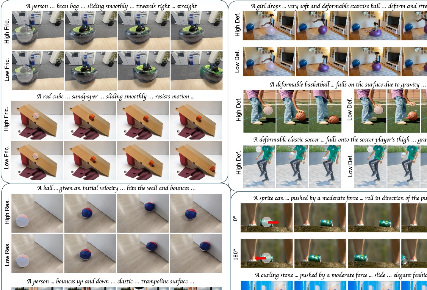
Pretrained video diffusion models render plausible textures and short-term motion but routinely violate physical constraints: bouncing objects fail to conserve a coherent coefficient of restitution, sliding objects ignore friction, and deformable bodies show inconsistent material response. Existing physics-aware approaches either rely on simulator-in-the-loop pipelines (expensive, geometry-dependent) or supervise a single attribute such as applied force (Force-Prompting). PhyCo targets continuous, interpretable, and compositional control over four physical axes — friction, restitution, deformation, and applied force — without invoking a simulator or explicit geometry at inference.
Method
PhyCo combines a curated simulation dataset with a two-stage training pipeline (Figure 2).
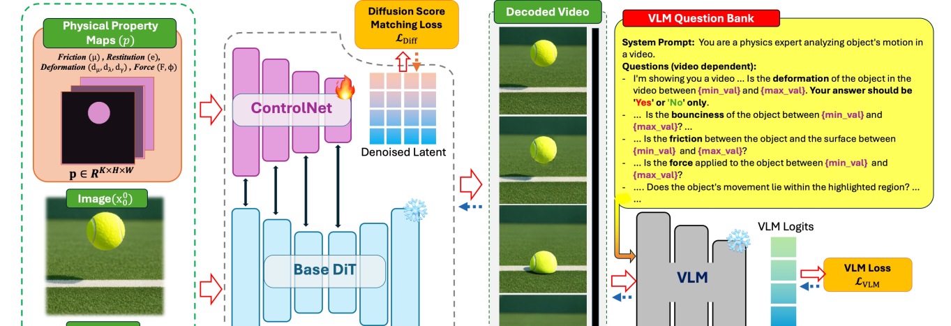
Dataset. Using Kubric, the authors generate >100K photorealistic clips spanning six (and ultimately eight) scenarios — brick on a plane, ball-wall rebound, vertical bouncing, soft ball under gravity, impact on a deformable body, and pool-table multi-ball collisions — each with randomized object color, surface material, camera placement, and 50 HDRI environments using Polyhaven textures (Figure 3). Crucially, each scene is constructed so that the controlled attribute manifests unambiguously in motion (a design constraint also identified by PISA and Force-Prompting); cluttered multi-object dynamics are deliberately avoided because they exceed the competence of current diffusion backbones and inject training variance unrelated to the physical signal.
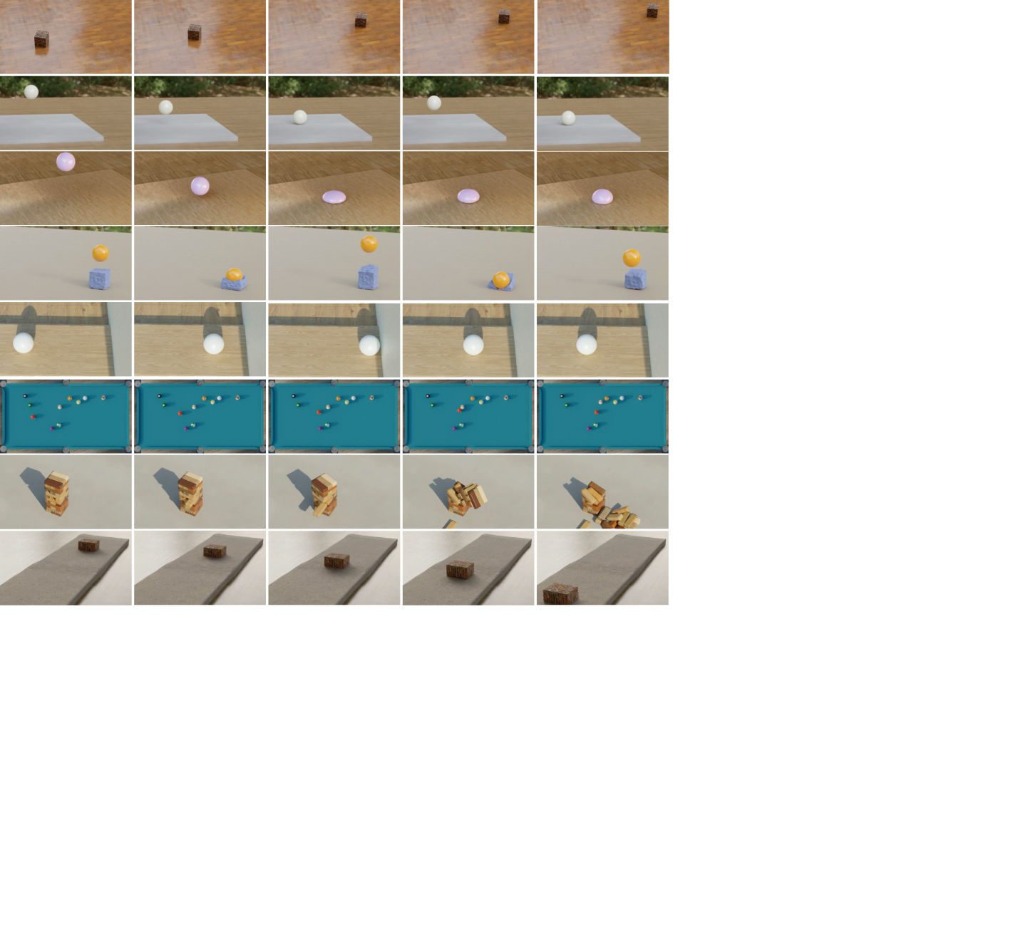
Stage 1 — Physics-supervised fine-tuning. A pretrained DiT (Cosmos-Predict2) is augmented with a ControlNet branch that takes pixel-aligned physical property maps as conditioning. These maps are spatial masks placing scalar values for friction, restitution, deformation, and force vectors at the relevant object locations (visible as the white blobs in Figure 4). The model is trained with the standard diffusion score-matching loss conditioned on these maps, so the network learns to associate the canonical visual signature of each property with its scalar value rather than memorizing scene-level appearance.
Stage 2 — VLM-guided reward optimization. A fine-tuned vision-language model is queried with targeted physics questions about each generated video (e.g., “did the ball rebound with the specified restitution?”) and produces differentiable feedback that is back-propagated as a reward signal on top of the ControlNet-conditioned generator. This stage sharpens quantitative adherence to the conditioning values rather than merely producing qualitatively plausible motion.
At inference, only the property maps and text are required — no physics engine, no mesh, no point cloud.
Results
On the Physics-IQ benchmark (Solid Mechanics, Fluid Dynamics, Optics, Magnetism, Thermodynamics; 396 reference videos), PhyCo improves over Cosmos-Predict2, CogVideoX-I2V-5B, SVD-XT, LTX-Video, Force-Prompting, and VLIPP across all categories, despite a train/test horizon mismatch (training on 57-frame clips vs. 120-frame benchmark sequences).
The synthetic ablation (Table 4) is the more mechanistic test, measuring per-attribute control error:
| Variant | FM ↓ | Fric. ↓ | FD (°) ↓ | Res. ↓ | Def. ↓ |
|---|---|---|---|---|---|
| Base (zero-shot) | 0.38 | 0.33 | 91.87 | 0.40 | 0.45 |
| Text-only fine-tuned | 0.31 | 0.30 | 40.35 | 0.31 | 0.14 |
| ControlNet (−VLM) | 0.33 | 0.24 | 38.05 | 0.28 | 0.14 |
| ControlNet (+VLM) | 0.28 | 0.20 | 22.53 | 0.16 | 0.10 |
Force-direction error drops from 91.87° (essentially random) to 22.53°, and restitution error halves from 0.31 to 0.16 when the VLM reward is added on top of the ControlNet. Notably, text-only fine-tuning on PhyCo data already cuts force-direction error to 40.35°, but cannot reach the spatial precision of pixel-aligned conditioning.
The 2AFC user study reinforces this: against CogVideoX-I2V-5B, PhyCo wins 95.5\% on friction, 100.0\% on restitution, 82.2\% on deformation, and 91.1\% on force; against Cosmos-Predict2B it wins 100.0\%, 93.2\%, 91.3\%, and 86.4\% respectively. Against Force-Prompting (force only), PhyCo wins 71.7\%. The text-only fine-tuned variant of PhyCo wins only 58.7\% on force and loses on deformation (56.8\% is borderline; restitution at 67.4\%), confirming that the ControlNet’s spatial conditioning — not just the dataset — drives the gains.
Limitations
The training distribution is restricted to visually clean, low-clutter scenes with isolated interactions; generalization to multi-object dense dynamics is explicitly out of scope and likely to degrade. The four physical axes are scalar abstractions — anisotropic friction, viscoelasticity, fracture, and fluid interactions are not modeled. Pixel-aligned property maps require the user (or an upstream module) to specify masks; the paper does not evaluate sensitivity to map noise or how property maps should be authored for novel objects. The 57-frame training horizon also caps the duration over which physical consistency is enforced, and the VLM reward inherits whatever biases its physics-querying prompts encode.
Why this matters
PhyCo demonstrates that physical controllability in video diffusion can be decoupled from simulator-in-the-loop inference: a ControlNet over scalar property maps plus VLM-derived differentiable feedback produces measurable, compositional control over friction, restitution, deformation, and force. The recipe — small, focused simulation suites that isolate canonical visual signatures, then RL-style refinement against a VLM critic — is a reusable template for grounding generative models in other structured priors.
Source: https://arxiv.org/abs/2604.28169
ViPO: Visual Preference Optimization at Scale
Problem
Preference optimization (DPO and its diffusion variants) has become standard for aligning visual generative models with human aesthetics, but unlike LLMs, the recipe has not scaled cleanly. Two coupled bottlenecks block progress. First, public preference datasets (Pick-a-Pic, HPDv2) are noisy in a structural sense: a “winner” image often beats the loser on aesthetic appeal but loses on prompt alignment or anatomy. Naively maximizing the DPO log-ratio on such samples pushes the model toward conflicting gradients. Second, the data themselves are stale — 512–768 px outputs from early SD-class models, with imbalanced prompt distributions and almost no video coverage. The paper attacks both: a noise-robust objective (Poly-DPO) and a reconstructed dataset (1M image pairs at 1024 px, 300K video pairs at 720p+).
Method: Poly-DPO
The Diffusion-DPO objective approximates the intractable preference likelihood on the denoising trajectory, yielding a loss of the form
\mathcal{L}_{\text{DPO}} = -\mathbb{E}\left[\log \sigma\left(-\beta T\, \Delta_\theta\right)\right],
where \Delta_\theta = \big(\|\epsilon_\theta(x^w_t)-\epsilon^w\|^2 - \|\epsilon_{\text{ref}}(x^w_t)-\epsilon^w\|^2\big) - \big(\|\epsilon_\theta(x^l_t)-\epsilon^l\|^2 - \|\epsilon_{\text{ref}}(x^l_t)-\epsilon^l\|^2\big) is the implicit reward margin between the winner w and loser l relative to a frozen reference. Under conflicting preferences, \Delta_\theta has inconsistent sign across dimensions; the sigmoid saturates and gradients on noisy pairs dominate.
Poly-DPO modulates the effective confidence by adding a polynomial term to the logit:
\mathcal{L}_{\text{Poly-DPO}} = -\mathbb{E}\left[\log \sigma\left(-\beta T\, \Delta_\theta - \alpha (\beta T \Delta_\theta)^k\right)\right],
controlled by a single exponent/scale hyperparameter (the authors emphasize “two new lines of code”). The polynomial term reshapes the loss landscape: for clean, consistent datasets it sharpens gradients on confident pairs; for biased datasets it dampens the contribution of pairs that would otherwise be over-confidently classified, preventing the model from over-fitting conflicting signals. Geometrically, this is a confidence-aware temperature on the implicit reward — similar in spirit to focal-loss style reweighting but applied to the DPO logit rather than to a classification probability.
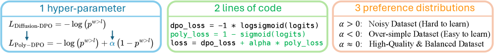
The same functional form covers three regimes (winner-dominant, loser-dominant, conflicting) by tuning one exponent, which is the practical selling point versus alternatives like IPO, KTO, or SPO that change the objective family.
Dataset: ViPO-Image-1M and ViPO-Video-300K
ViPO-Image-1M contains 1M pairs at 1024 px, generated by FLUX and Qwen-Image, organized into five categories (general aesthetics, prompt alignment, anatomy, text rendering, style). ViPO-Video-300K provides 300K pairs at 720p+ from WanVideo and Seedance across three categories. The construction explicitly enforces balanced category coverage rather than the random sampling that lets “easy” aesthetic preferences dominate Pick-a-Pic.
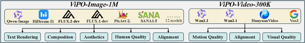
Pairs are produced by sampling multiple candidates per prompt from the SOTA generators and ranking with category-specific scorers (full pipeline deferred to the appendix). The key design claim is that using current-generation models eliminates a confound in older datasets, where the “winner” can still be objectively poor by 2024 standards, blunting the alignment signal.
Results
The headline experiment evaluates clean scaling. Across SD1.5, SDXL, SD3, SD3.5-Medium, and FLUX, training on ViPO-Image-1M with Poly-DPO yields monotone improvements in win rate as data scales, in contrast to Diffusion-DPO on Pick-a-Pic-v2, which plateaus or regresses.
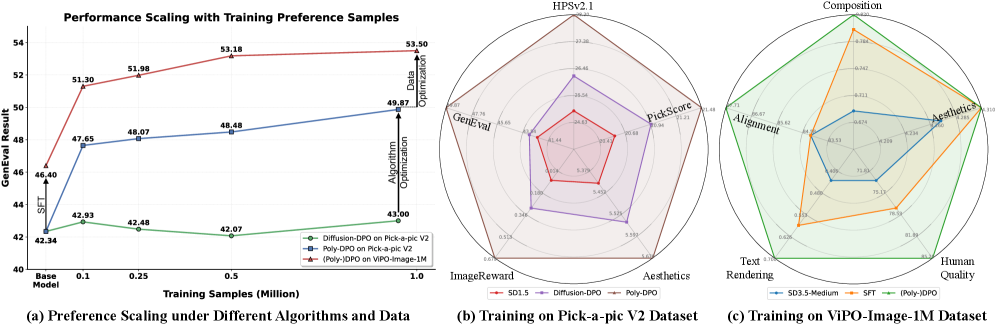
On the biased-data stress test (training SD1.5 on Pick-a-Pic-v2), Poly-DPO outperforms Diffusion-DPO across every evaluation dimension — aesthetics, alignment, and structural quality (Figure 1b). For SD3.5-Medium trained on ViPO-Image-1M, the model improves uniformly across all evaluation axes (Figure 1c) rather than trading one dimension for another, which is the failure mode of vanilla DPO on noisy data. Video results on Wan2.1-T2V-1.3B trained on ViPO-Video-300K extend the same conclusion to the temporal setting.
Limitations and open questions
The abstract is truncated and exact win-rate numbers are not in the supplied excerpts, so the magnitude of improvement vs. SPO/IPO/MaPO baselines cannot be quoted precisely from the provided text. The polynomial term introduces a hyperparameter whose optimum depends on dataset noise level — there is no principled estimator given. The pipeline still relies on automated scorers to label pairs, inheriting their biases (e.g., HPS, PickScore failure modes on text rendering and anatomy). Whether Poly-DPO confers benefits beyond the saturation regime of \beta tuning, or simply re-discovers a better effective \beta schedule, is not disentangled. Finally, the dataset is generated by FLUX/Qwen-Image/WanVideo/Seedance, so distillation-style ceilings on the student likely apply.
Why this matters
If preference optimization for visual generation is to follow the LLM trajectory, both the objective and the data must scale gracefully under noise. ViPO offers a minimal-edit objective change plus a clean, large, high-resolution preference corpus — the combination needed to make DPO-style alignment a reliable scaling axis for image and video models rather than a brittle finetuning trick.
Source: https://arxiv.org/abs/2604.24953
Heterogeneous Scientific Foundation Model Collaboration
Problem
Agentic LLM systems treat language as the universal interface, which forces all reasoning to pass through textualized representations. This is a poor fit for scientific tasks whose inputs live in non-linguistic modalities (time series, tabular data, molecular structure, geospatial fields) and where strong domain-specific foundation models (FMs) already exist but lack a native language API. The paper formalizes the gap and proposes Eywa, a framework that lets an LLM orchestrate specialist FMs as first-class participants rather than as tools-of-last-resort hidden behind text serialization.
Formally, a task is \tau=(q,x,y^\star,\ell) with input factorization \mathcal{X}=\mathcal{X}_{\mathrm{lng}}\times\mathcal{X}_1\times\cdots\times\mathcal{X}_m, where \mathcal{X}_k is the native input space of FM F_k:\mathcal{X}_k\times\mathcal{U}_k\to\mathcal{O}_k. The agentic system G minimizes \mathbb{E}_{\tau}[\ell(G(q,x),y^\star)]. The LLM is a policy A_{\mathrm{LLM}}:\mathcal{S}\to\Delta(\mathcal{M}) that can only observe x_k through some textual projection — which is the source of information loss the framework is built to remove.
Method
EywaAgent (FM–LLM “Tsaheylu” bond). For each domain k, Eywa defines an interface pair (\phi_k,\psi_k):
- \phi_k:\mathcal{S}\to\mathcal{U}_k — a query compiler that turns the LLM’s task state s into a structured FM invocation (dataset id, conditioning variables, horizon, hyperparameters).
- \psi_k:\mathcal{O}_k\to\mathcal{Z}_k — a response adapter that lifts the FM’s raw output o_k into a structured, language-consumable context z_k (summary statistics, calibrated forecasts, ranked candidates, etc.).
The end-to-end loop is \tau \xrightarrow{A_{\mathrm{LLM}}} s \xrightarrow{\phi_k} u_k \xrightarrow{F_k} o_k \xrightarrow{\psi_k} z_k \xrightarrow{A_{\mathrm{LLM}}} \hat{y}.
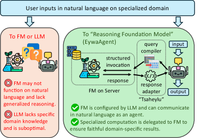
The interface is implemented over the Model Context Protocol: each F_k is exposed as a remote service with a typed schema for \mathcal{U}_k,\mathcal{O}_k. The MCP server retrieves x_k, runs F_k(x_k,u_k), and returns a structured o_k; \psi_k is then a deterministic adapter (templated JSON-to-text plus numeric digesting) appended to the LLM context.
EywaMAS. Extends the single-agent design to a multi-agent system \mathcal{M}_{\mathrm{Eywa}}=(\mathcal{A},\mathcal{G}) where \mathcal{A} mixes plain LLM agents and EywaAgents under topology \mathcal{G}. The state/message dynamics are the standard s_i^{(t)} = \mathrm{Update}_i(s_i^{(t-1)},m_{-i}^{(t)}),\quad m_i^{(t)}\sim A_i(s_i^{(t)}), so any existing planner/worker/summarizer architecture can be upgraded by swapping language-only workers for EywaAgents without changing the protocol. When all agents are LLMs, EywaMAS reduces to a conventional MAS.
EywaOrchestra. A planner-driven orchestration layer that dynamically chooses which agents to invoke and in what order, replacing fixed topologies with structured plans over the agent pool.
Results
Eywabench covers 9 sub-domains across physical, life, and social science, spanning text, time series, and tabular modalities, built from DeepPrinciple, MMLU-Pro, fev-bench, and TabArena.
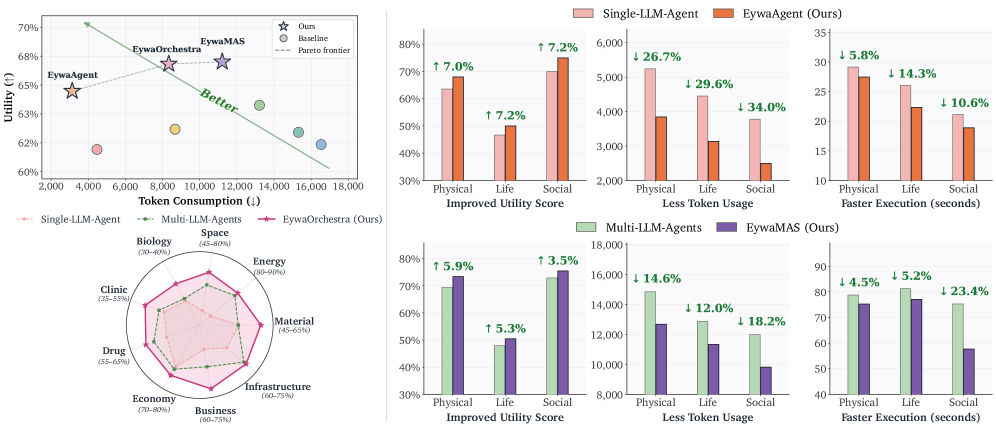
Single-agent comparison (overall utility / time / tokens):
- Single-LLM-Agent: 0.6154 / 25.22 s / 4469
- EywaAgent: 0.6558 / 22.78 s / 3137
Per-domain, EywaAgent improves utility on every sub-domain — e.g., Energy 0.8202→0.8390, Space 0.5235→0.6123, Biology 0.3402→0.3718, Drug 0.6004→0.6199, Business 0.6528→0.7371. Token consumption drops roughly 30% (4469→3137) because numerical reasoning is offloaded to FMs rather than emulated in-context.
Multi-agent comparison (overall utility):
- Refine MAS: 0.6294 at 60.59 s / 8673 tokens
- Debate MAS: 0.6460 at 78.22 s / 13.6k–16.7k tokens
- EywaAgent (single agent) already exceeds both at 0.6558 with ~3× less wall-clock and ~3–5× fewer tokens.
The Debate baseline pays a heavy efficiency cost on time-series-heavy domains (Biology 101.64 s, Economy 92.72 s) without commensurate utility gains, indicating that more language-only deliberation does not substitute for direct FM access.
Limitations and open questions
- The “domain advantage” assumption is treated axiomatically; the framework provides no mechanism to detect when an FM is miscalibrated or out-of-distribution, and the LLM has limited means to second-guess o_k.
- Adapter design (\phi_k,\psi_k) is hand-engineered per FM. Scaling to dozens of specialists likely requires learned or auto-generated adapters, and the response adapter \psi_k is a lossy bottleneck that the paper does not analyze.
- Orchestration evaluation in the provided sections is partial; the planning policy in EywaOrchestra is not characterized in terms of regret or planning horizon.
- Eywabench overlaps with its source datasets (TabArena, fev-bench), so contamination relative to LLM pretraining is not controlled.
- Robustness to FM disagreement, FM failure modes, and adversarial u_k configurations is unaddressed.
Why this matters
Most “scientific agent” work routes specialist computation through brittle textual tool-use; Eywa formalizes the FM as a typed, MCP-exposed callable with explicit query/response adapters, and shows that this alone yields better utility at lower token and latency cost than larger language-only multi-agent stacks. The interesting research surface this opens is learning (\phi_k,\psi_k) end-to-end and reasoning under FM uncertainty, rather than scaling LLM deliberation.
Source: https://arxiv.org/abs/2604.27351
Hacker News Signals
Refusal in Language Models Is Mediated by a Single Direction
Source: https://arxiv.org/abs/2406.11717
This paper identifies a one-dimensional linear subspace in residual stream activations that causally mediates refusal behavior across a range of open-weight instruction-tuned LLMs (Llama-3, Mistral, Gemma, Qwen, etc.). The core finding: there exists a single direction \hat{r} \in \mathbb{R}^d such that projecting out this direction from all residual stream activations during inference — across every layer — reliably ablates refusal without measurably degrading general capability.
The direction is identified via contrastive mean-differencing: collect activations on harmful vs. harmless prompts, compute \hat{r} = \text{normalize}(\mu_\text{harmful} - \mu_\text{harmless}), then apply the intervention \mathbf{x} \leftarrow \mathbf{x} - (\mathbf{x} \cdot \hat{r})\hat{r} at every residual stream position. The authors also show the direction can be used in the opposite direction — adding a scaled multiple of \hat{r} to activations causes the model to refuse benign prompts.
A complementary finding is that refusal can be induced or eliminated by targeting a single weight matrix via direct weight edits: specifically, adding \alpha \hat{r} \hat{r}^\top to W_O of attention layers. This is a rank-1 edit, more interpretable than full fine-tune approaches like LoRA-based jailbreaks.
The work connects to prior linear representation hypothesis literature and provides empirical support that safety fine-tuning writes a low-dimensional feature rather than a distributed circuit. This has both practical consequences (cheap bypass) and theoretical ones: alignment via RLHF is encoding a nearly 1D decision boundary in a very high-dimensional space. The authors benchmark refusal rates on JailbreakBench and show >95% attack success after ablation with minimal MT-Bench degradation. Limitations: the analysis is restricted to open-weight models where activations are accessible, and it is unclear whether the same direction generalizes across architectures at the feature level or just functionally.
Alignment Whack-a-Mole: Finetuning Activates Recall of Copyrighted Books in LLMs
Source: https://github.com/cauchy221/Alignment-Whack-a-Mole-Code
This repository accompanies research showing that safety-aligned LLMs that refuse to reproduce copyrighted text can be made to recall that text through lightweight fine-tuning — even when the fine-tuning data is entirely unrelated to the target books. The “whack-a-mole” framing captures the core problem: suppressing one undesired behavior via alignment destabilizes others, and fine-tuning restores the suppressed capability.
The mechanism is consistent with the linear representation picture from the refusal-direction paper above. Safety alignment suppresses memorized content via directions or inhibitory circuits in the residual stream; a few gradient steps on benign data shift the model’s activation distribution enough to partially undo that suppression. Crucially, the effect does not require targeted attacks — even benign fine-tuning on instruction-following data re-enables verbatim recall of Harry Potter, The Great Gatsby, and other tested texts.
The evaluation protocol measures verbatim extraction rate using exact n-gram match (n=50) and ROUGE-L against ground-truth passages, comparing base, aligned, and fine-tuned-aligned models. Results show aligned models reduce extraction rates substantially, but 100–500 gradient steps of unrelated fine-tuning brings extraction rates close to the base model’s levels.
This is technically significant because it challenges the assumption that post-training can create a stable partition between “will recall” and “won’t recall.” The memorization exists in the weights regardless of alignment; alignment appears to add a learned gate rather than erase the content. From a copyright-liability perspective this matters for API providers who claim their aligned models do not reproduce training data. Open questions include whether larger models memorize more robustly (making the gate easier to bypass), and whether any training-time intervention can actually remove memorized content rather than gate it.
AI Self-preferencing in Algorithmic Hiring: Empirical Evidence and Insights
Source: https://arxiv.org/abs/2509.00462
This paper tests whether LLM-based hiring systems exhibit self-preferencing — systematically ranking candidates higher when those candidates’ resumes indicate they were generated or optimized with AI assistance, or when candidates signal AI proficiency in ways that correlate with the evaluating model’s training distribution. The problem matters because algorithmic hiring is already deployed at scale, and systematic bias in ranking has legal and labor-market consequences.
The experimental design uses a controlled resume audit: a factorial design varying candidate qualifications, AI-signal language (e.g., mentioning GPT-4, Copilot, or model-specific tools), and evaluating model identity. Resumes are scored by multiple LLMs (GPT-4o, Claude 3.5, Gemini 1.5 Pro, Llama 3). The key finding is statistically significant self-preferencing: models assign higher scores to resumes that mention tools or workflows associated with the evaluating model’s own ecosystem. GPT-4o scores resumes mentioning OpenAI tools roughly 8–12 percentile points higher than equivalent resumes mentioning competing tools, controlling for all other factors.
The mechanism hypothesized is that LLMs trained on internet data absorb implicit brand-sentiment associations, and evaluation prompts activate these associations during scoring. This is not a simple keyword-match artifact — the effect persists when tool names are paraphrased or described functionally.
Limitations are substantial: resume audit studies have limited external validity, the effect size may be smaller in real deployments with human-in-the-loop review, and causal attribution to specific training data is not possible from behavioral experiments alone. The paper does not propose a debiasing fix, though contrastive decoding or calibration against a neutral baseline are natural candidates. The open question is whether fine-tuning for hiring use cases amplifies or attenuates self-preferencing.
Shai-Hulud Themed Malware Found in the PyTorch Lightning AI Training Library
Source: https://semgrep.dev/blog/2026/malicious-dependency-in-pytorch-lightning-used-for-ai-training/
Semgrep’s security team identified a malicious package in the PyTorch Lightning dependency tree. The package used Dune-themed variable and function names — referencing “Shai-Hulud” (sandworm) — apparently as obfuscation-by-novelty to avoid pattern-matching detectors tuned to common malware strings.
The technical substance is a supply-chain attack variant. The malicious dependency was a typosquat or dependency-confusion package that, when installed, executed a post-install hook (setup.py or pyproject.toml build script) to run arbitrary code. The payload’s Dune-themed naming is cosmetic; the functional behavior is standard infostealer/remote-access-trojan territory: exfiltrating environment variables (which in ML training environments commonly contain API keys, cloud credentials, Hugging Face tokens, and wandb secrets), and establishing a callback channel.
The ML-specific threat surface is worth noting. Training jobs routinely run in cloud VMs or Kubernetes pods with broad IAM roles, access to model registries, and environment variables containing secrets for S3/GCS/Azure storage. A compromised training environment can exfiltrate model weights, training data, and credentials in a single job run. The torch.hub and Hugging Face from_pretrained ecosystems also represent additional vectors since they execute remote code by design.
Detection in this case required static analysis of the dependency graph — Semgrep’s rules flagged the post-install execution. Mitigations include pinning dependency hashes in requirements.txt or pyproject.toml, running installs in network-isolated environments, and auditing setup.py for subprocess/socket calls before execution. The broader issue is that the ML tooling ecosystem has grown faster than its security review processes, and popular training frameworks accumulate large transitive dependency trees with minimal vetting.
The IBM Granite 4.1 Family of Models
Source: https://research.ibm.com/blog/granite-4-1-ai-foundation-models
IBM’s Granite 4.1 release updates the dense and MoE variants in their enterprise-focused open-weights family. The technical points of interest are the architectural and training changes relative to Granite 3.x.
Granite 4.1 adopts a hybrid attention architecture combining full attention layers with sliding-window local attention layers, reducing the quadratic attention cost for long-context processing. The context window extends to 128K tokens. The MoE variant (Granite 4.1 MoE) uses a top-k sparse routing mechanism with load-balancing auxiliary loss — standard practice since Mixtral — but IBM reports tuning the expert granularity and count specifically for inference efficiency on their internal hardware targets.
Training data composition is disclosed at a higher level than most releases: the blog reports a mix weighted toward code, technical documents, and enterprise data domains, with explicit filtering for license-compatible content — a differentiator IBM has consistently emphasized for enterprise IP-risk reasons. The instruct variants are trained with a multi-stage pipeline: SFT on curated instruction data, then DPO rather than PPO-based RLHF.
Benchmark numbers reported include MMLU (70B-class dense model: ~84%), HumanEval (~78%), and long-context retrieval (NIAH at 128K: >95% recall). The small dense models (3B, 8B) are positioned for on-device and edge deployment with claimed competitive performance against Llama 3.1 8B on coding tasks.
Limitations: the blog post is not a technical report, so architectural hyperparameters, training compute, and full benchmark methodology are not disclosed. The MoE expert count and routing details are not specified. Whether the hybrid attention pattern is determined by a fixed interleaving ratio or learned is unclear.
LFM2-24B-A2B: Scaling Up the LFM2 Architecture
Source: https://www.liquid.ai/blog/lfm2-24b-a2b
Liquid AI’s LFM2-24B-A2B is a 24B total parameter model with 2B active parameters per forward pass, scaling up their LFM2 architecture which combines structured state-space model (SSM) layers with attention layers in a hybrid configuration. The “A2B” designation refers to the 2B active parameter count under MoE sparse routing.
The LFM2 architecture uses Liquid Foundation Model layers — a variant of the linear recurrence / structured SSM family (related to Mamba/S6 or RWKV-style formulations) — interleaved with grouped-query attention. The recurrence enables O(1) per-step inference cost for the SSM layers once the recurrent state is populated, which is the primary motivation: long sequences are processed with sub-quadratic cost. The 24B/2B MoE configuration then layers sparse routing on top, so most parameters are dormant per token, keeping FLOPs close to a 2B dense model.
The reported benchmark results show competitive performance with models in the 7B-13B dense range on standard evals: MMLU ~72%, MATH ~58%, and notably strong performance on long-context tasks where the SSM recurrence provides architectural advantage. Throughput benchmarks claim 2-4x tokens/sec improvement over a 7B dense transformer at equivalent quality on sequence lengths >32K.
Key open questions: SSM-attention hybrids have shown training instabilities at scale that pure-transformer models avoid; the blog does not discuss loss curves or training stability interventions. The LFM layer formulation is not fully specified in the post — the relationship to specific SSM variants (S4, Mamba, GLA) is not made precise. Evaluation on tasks requiring genuine long-range reasoning (rather than retrieval) remains the meaningful test for SSM-based architectures. Weights are released, which enables independent architectural analysis.
Noteworthy New Repositories
atomicarchitects/equiformer_v3
Equiformer V3 is the third generation of the EquiformerV2 architecture for atomistic machine learning, targeting molecular property prediction and relaxation tasks on benchmarks such as OC20 and OC22. The core design retains SE(3)/E(3)-equivariant graph attention built on irreducible representations (irreps) of SO(3), with spherical harmonics as angular basis functions and radial networks conditioning interaction weights. V3 introduces architectural refinements to the attention mechanism and tensor product contractions that improve parameter efficiency while preserving equivariance. The network processes atomic graphs where each node carries a feature vector decomposed into irreps channels \bigoplus_l (2l+1)-dimensional components, and edges carry geometric embeddings derived from relative positions. Message passing respects group equivariance by construction, so predictions of forces and energies transform correctly under rotation and reflection. The repository ships training configs, pretrained checkpoints, and evaluation scripts against the Open Catalyst datasets. Compared to EquiformerV2, V3 targets better scaling behavior with respect to model depth and system size, reducing the computational cost of the Clebsch-Gordan tensor products that dominate runtime. Of interest to anyone working on equivariant neural potentials or foundation models for materials science.
Source: https://github.com/atomicarchitects/equiformer_v3
future-agi/future-agi
Future-AGI is an open-source evaluation and observability framework for LLM-based pipelines and agents. The technical core is a suite of model-agnostic quality metrics — covering factual consistency, instruction following, context faithfulness, and hallucination detection — that can be run either locally or through a hosted API. Metrics are computed by a combination of reference-free LLM judges and deterministic heuristics, with configurable thresholds to gate pipeline stages. The repo provides a Python SDK for instrumenting arbitrary LangChain, LlamaIndex, or raw API call graphs, capturing input/output traces that are then scored asynchronously. A Pydantic-based schema defines the trace structure, enabling typed integrations and downstream aggregation. Evaluation results feed into a dashboard for monitoring score drift across model versions and prompt changes. The framework also supports dataset-level batch evaluation, where a test set is scored and results are exported as structured reports. Unlike closed observability products, the metric computation code is inspectable and extensible — users can register custom evaluators conforming to a simple interface. The primary limitation is that judge-based metrics inherit the biases and capability ceiling of the underlying judge model; no ground-truth calibration data is currently shipped with the repo.
Source: https://github.com/future-agi/future-agi
Tisha-runwal/Personalized-Federated-Learning-for-Privacy–Preserving-and-Scalable-IoT-Driven-Smart-Healthcare
This repository implements a personalized federated learning (pFL) system designed for heterogeneous IoT health-monitoring devices. The core algorithm is a variant of per-FedAvg or local fine-tuning federated learning, where a global model is aggregated via FedAvg across participating clients (representing individual patient devices), then each client adapts the global weights with a small number of local gradient steps on private on-device data. This two-stage approach targets the statistical heterogeneity endemic to healthcare IoT, where sensor distributions and pathology prevalence differ sharply across patients. Privacy is enforced via differential privacy (DP) noise injection during local gradient computation before upload, with a configurable privacy budget (\epsilon, \delta). The codebase includes simulation infrastructure for partitioning standard health datasets (e.g., MIMIC-derived vitals or ECG benchmarks) into non-IID client splits using Dirichlet allocation with concentration parameter \alpha. Communication efficiency is addressed through gradient sparsification before aggregation. The repo contains training scripts, client/server simulation using Flower or a lightweight custom coordinator, and evaluation scripts measuring both global and per-client personalized accuracy. Scalability analysis under varying numbers of simulated clients is included. Primary limitations: experiments are simulation-only with no real embedded deployment, and the DP accounting uses basic composition rather than tighter RDP bounds.
FonaTech/Project_Chronos
Project Chronos is a time-series forecasting framework oriented toward long-horizon prediction under distributional shift. The architecture centers on a transformer encoder-decoder with learned temporal positional encodings that explicitly separate trend, seasonality, and residual decomposition within the embedding stage, drawing on approaches similar to Autoformer or FEDformer but with a modular component structure that makes swapping decomposition strategies straightforward. The patching strategy divides input sequences into non-overlapping windows before tokenization, reducing the quadratic attention cost for long contexts. The framework supports probabilistic forecasting by outputting parameters of a target distribution (Gaussian or Student-t) rather than point predictions, enabling calibrated uncertainty quantification via proper scoring rules. Training infrastructure includes a curriculum schedule that progressively increases forecast horizon length, which stabilizes gradient flow for very long prediction windows. The repo targets multivariate settings and includes connectors for common time-series datasets (ETT, Weather, Traffic) as well as a generic CSV loader. Configuration is handled through YAML files controlling model depth, patch size, decomposition type, and distributional head. Evaluation scripts compute MAE, MSE, CRPS, and calibration metrics. The main open question is systematic benchmarking against established baselines such as PatchTST or iTransformer at equivalent parameter budgets.
Source: https://github.com/FonaTech/Project_Chronos
Dynamis-Labs/spectralquant
SpectralQuant is a library for spectral analysis and quantization of neural network weight matrices, framing model compression as a problem in numerical linear algebra rather than purely magnitude-based pruning. The core operation is a truncated SVD decomposition of weight matrices W \approx U_k \Sigma_k V_k^\top, where the rank k is chosen per-layer by a configurable energy retention threshold on the singular value spectrum. This low-rank approximation is combined with quantization of the retained singular vectors and values, enabling a two-axis compression scheme that jointly reduces both rank and numerical precision. The library includes routines for analyzing the singular value decay profile of pretrained models, which can diagnose layers with fast spectral decay (high compressibility) versus flat spectra (resistant to low-rank approximation). Supported backends include PyTorch, with hooks that replace nn.Linear layers in-place after decomposition. Post-compression fine-tuning utilities are provided to recover accuracy lost from truncation. The repo includes benchmarks on standard vision and language models measuring compression ratio versus accuracy tradeoff curves. A known limitation is that the SVD-based approach is most effective for fully connected and attention projection layers; convolutional layers require reshape heuristics that can degrade decomposition quality.
Source: https://github.com/Dynamis-Labs/spectralquant
facebookresearch/neuroai
Facebook Research’s NeuroAI repository collects computational tools and model implementations at the intersection of systems neuroscience and artificial intelligence. The technical content spans two directions: using neural data to benchmark and constrain AI models, and using AI models as functional hypotheses about neural computation. The library provides utilities for fitting representational similarity analysis (RSA) and centered kernel alignment (CKA) between neural population recordings and DNN intermediate activations, quantifying the degree to which a model’s representational geometry matches brain area responses. It also includes implementations of task-optimized neural network models (e.g., ventral stream CNNs, recurrent circuits for working memory) alongside data loaders for standard neural benchmarks such as NeuralBench or Brain-Score compatible evaluation interfaces. Predictivity metrics are computed using linear regression or partial least squares mapping from model activations to neural firing rates, with cross-validation over held-out trials. On the AI-to-neuro direction, the repo ships analysis tools for probing emergent properties of large pretrained vision and language models — for instance, localizing units selective for faces, objects, or syntax. The codebase is modular: neural data handling, model probing, and metric computation are separated into independent subpackages. A limitation is that documentation for the neural data loading pipeline assumes familiarity with specific proprietary dataset formats.