Daily AI Digest — 2026-10-05
arXiv Highlights
Does Learning Protein Folding Generalize to Broader Reasoning?
The paper asks whether training a frozen LLM on protein-structure-derived question-answer pairs, with an auxiliary 3D geometry readout, yields reusable reasoning primitives that transfer to graph, spatial, scientific, and mixed reasoning benchmarks with no protein content at inference. The motivation is that one solved structure deterministically generates thousands of exactly checkable spatial-topological statements, giving dense ground-truth supervision for the kind of relational reasoning that web text underspecifies.
Setup and training signal
The base model is Qwen3.5-9B, frozen, with LoRA (rank 16, \alpha=32, dropout 0.05, 43.28M trainable params) on audited attention and FFN projections. For a protein of length L with backbone coordinates Y \in \mathbb{R}^{L\times 4\times 3}, the model consumes a prompt with one marker token per residue and produces residue states
H = f_\theta(x)_{\mathrm{res}} \in \mathbb{R}^{L\times 4096}.
Coordinates Y are never fed as input; they only generate labels and a continuous geometry supervision signal through a shared workspace (3.90M params) and a frozen decoder (3.31M). FoldingCorpus packs 12 programmatic questions per protein — contact (C_\alpha < 8 Å, sequence separation \geq 6), distance comparison, segment orientation, center proximity, local direction, chirality, multi-constraint, and a 32-way global-summary match. Nine are binary, two three-way, one 32-way; every option is a single vocabulary token so supervision is ordinary next-token cross-entropy on the native LM head.
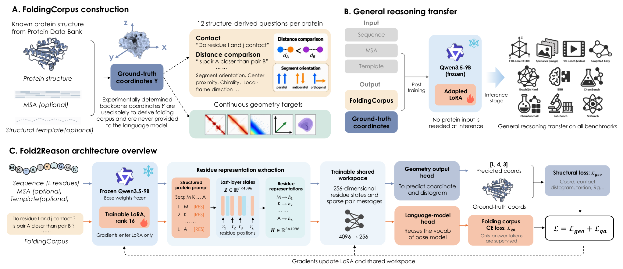
Training uses 1,000 proteins (lengths 29–199) across sequence-only, sequence+MSA, and sequence+MSA+template views, yielding 12,000 records packed as one example per protein. The entire run is three epochs / 375 optimizer steps on 4×A800-80G, three seeds, no benchmark-based checkpoint selection.
Main transfer result
On the General-10 suite (spatial, graph, scientific, mixed), Fold2Reason raises macro accuracy from 45.09% to 48.33% (+3.23 pp, SD 0.15 pp over seeds). All 10 benchmarks improve. Largest gains: GraphQA Hard +6.83 pp, SpatialViz +6.10 pp, GraphQA Easy +4.56 pp, ChemBench4K +4.37 pp, BBH +2.36 pp. The seven text-only datasets (excluding image/graph-visual ones) still gain +2.93 pp macro, and after removing GraphQA Easy/Hard the eight-dataset macro gain is +2.62 pp — the effect is not localized to graph-like formats.
Crucially, structure prediction itself improves 2.7–3.5× over the base model on FoldBench, confirming that the LoRA’d backbone genuinely acquires geometric competence rather than merely learning question formats.
Matched controls
The core causal claim rests on three Pure-LoRA controls sharing the base model, 12-question packing, 375 steps, and seeds:
- Hidden Geometry: keeps real protein prompts but recomputes answers from an unobserved random point structure. Gain: +0.92 pp. Internally coherent but input-decoupled geometry gives weak transfer.
- Format Copy: donor answer codes copied without geometric grounding. Change: −0.09 pp.
- Fixed Shuffle: original prompts, donor labels matched only by operator/vocabulary. Change: −0.27 pp.
Fold2Reason’s +3.23 pp is more than 3× the strongest control, so the benefit is not attributable to answer-token priors, format exposure, or supervised-token budget. The ordering (real geometry ≫ coherent-but-unrelated geometry ≫ shuffled) is the paper’s cleanest evidence that it is the correspondence between protein input and spatial target that produces transferable structure.
Structural fidelity
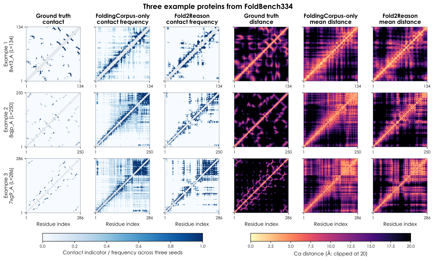
The contact and distance maps on FoldBench334 show that Fold2Reason produces visibly sharper diagonals and long-range contacts than a FoldingCorpus-only ablation, consistent with the quantitative 2.7–3.5× scaling. The improvement persists at L=286, outside the 29–199 training length range, suggesting the geometric representation is not just memorized length-conditioned templates.
Scale and family generalization
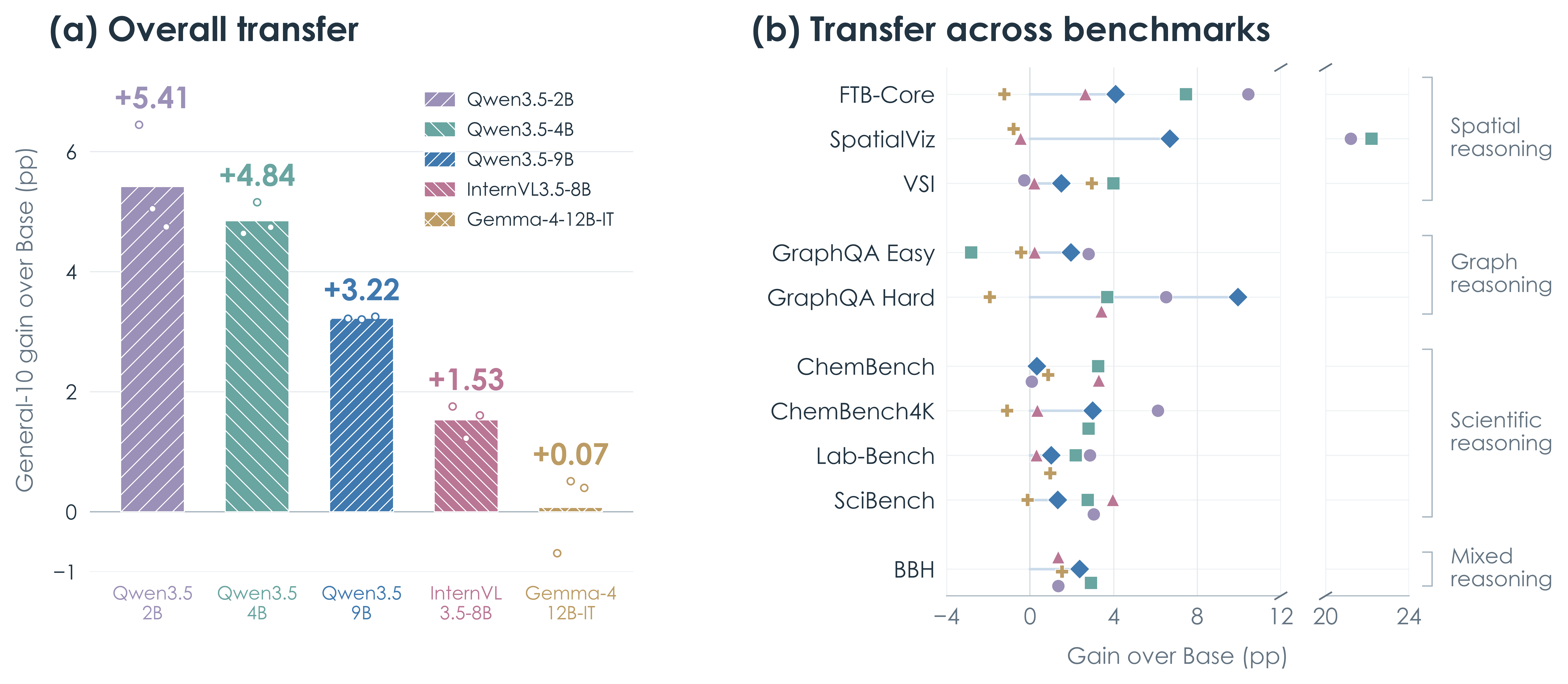
The per-benchmark breakdown across model sizes/families shows consistent positive mean changes, though with large SpatialViz-dominated variance; the paper breaks the horizontal axis to accommodate it. This weakens the “Qwen3.5-9B is a special case” worry but the figure also makes clear that gains are concentrated in spatial and graph tasks for every backbone.
Limitations and open questions
The training corpus is tiny (1,000 proteins, 375 steps), so the ceiling of this effect is unknown — does scaling the structure dataset push the macro gain further, or saturate? Second, the proteins are short (L \leq 199), MSA/template conditioning is mixed in, and the frozen decoder protocol in Appendix E matters for whether the geometric signal is genuinely flowing through the LLM’s representations rather than being captured by the workspace. Third, SciBench (+1.03 pp) and Lab-Bench (+0.64 pp) move much less than graph/spatial benchmarks, so “general reasoning” is overstated: the transfer looks concentrated in relational-spatial-combinatorial tasks that structurally resemble the pretext. Fourth, the parsing audit in Appendix H.1 flags residual answer-selection bias on FTB-Core and SpatialViz. Finally, the controls isolate correspondence vs. format but not whether the gain comes from the discrete QA head, the continuous geometry decoder, or their interaction — an ablation separating those two signals would be the natural next experiment.
Why this matters
Non-linguistic, deterministically verifiable supervision from a physical domain (protein geometry) measurably improves an LLM on unrelated spatial and graph reasoning, with carefully matched controls ruling out format/label-token effects. If this holds at scale, it suggests a general recipe for injecting relational competence into LLMs using any domain where ground truth is computable rather than scraped.
Source: https://arxiv.org/abs/2609.38879
Scaling Trajectories for Complex Tasks through Recursive Self-Rewrite
Problem
Agentic LLMs trained on successful trajectories typically rely on specialized scaffolds — progress trackers, retry wrappers, state managers, verifier-aware controllers — that are not available at deployment. The usual options are unsatisfactory: either restrict data collection to a single general harness and lose coverage on hard tasks, or train on harness-dependent trajectories and inherit interventions the deployed agent cannot reproduce. Recursive Self-Rewrite (RSR) targets this gap: use many harnesses to discover solutions, then rewrite them into trajectories executable under a single general harness, screening out any leakage of harness-specific affordances.
Method
RSR uses one base model (Qwen-3.8-27B) in three roles across three stages.
Stage 1 — Multi-harness discovery. The same base model is run against a terminal task pool under several harnesses that differ in control structure (progress tracking, continuation across context breaks, state checkpointing, validator-driven recovery, etc.). Successful trajectories are collected per harness. The joint coverage across three harnesses on roughly 3K tasks is 759 solved tasks, which is 34.3% more than the strongest single harness — concrete evidence that harness diversity expands the solvable set rather than merely reshuffling it.
Stage 2 — Rewrite under a general harness. Each successful source trajectory is reconstructed into one or more general-harness demonstrations using three roles:
- Planner: abstracts the trajectory into a runbook — a procedure describing the task-solving steps independent of harness-specific affordances.
- Critic: audits the runbook and the proposed rewrite for two failure modes: (i) verifier leakage, where the solution encodes knowledge of the grading check (e.g., writing exactly the string the verifier greps), and (ii) solution leakage, where harness-provided state or hints appear as if the executor produced them. The critic drives recursive revision: runbooks are iteratively rewritten until they pass the audit, which is the “recursive” element of the name.
- Executor: runs the qualified runbook in a fresh sandbox under the general harness, producing a candidate trajectory that is verified end-to-end.
Only trajectories that both (a) pass critic screening and (b) are reproduced successfully by the executor under the general harness are retained for SFT.
Stage 3 — SFT and iteration. From 2,001 successful source trajectories, RSR expands to 11,094 rewritten training trajectories (≈5.5× amplification, since each source can yield multiple valid rewrites). The base model is finetuned on these.
Task pool
The training pool is ~3K terminal tasks: ~2.5K self-constructed SWR tasks across 50 domains (software usage, biology, chemistry, physics, hardware, operations, security) plus 420 filtered-and-hardened tasks adapted from RST. The domain breadth is important: it forces the planner/critic to generalize the runbook abstraction across tool-use regimes rather than overfitting to shell idioms.
Results
Pass@3 improvements over the base model after RSR SFT:
- Terminal-Bench 2: 57.0% → 74.2% (+17.2 points)
- Terminal-Bench 4: 1.5% → 9.1% (6× relative; absolute still low, indicating headroom)
- Terminal-Bench Hard (self-curated): 39.0% → 63.0% (+24.0 points)
- Software Terminal (self-curated): 3.0% → 6.0% (2× relative)
The paper also reports that RSR beats direct trajectory SFT — i.e., finetuning on the original harness-assisted trajectories without rewriting. This is the key ablation: it isolates the value of the rewrite+audit pipeline from the value of simply having harder solved tasks in the training set. The gap suggests that direct SFT either (i) teaches the model to expect harness interventions that aren’t there at eval time, or (ii) absorbs verifier/solution leakage that doesn’t transfer.
Limitations and open questions
- Terminal-Bench 4 at 9.1% and Software Terminal at 6.0% remain low in absolute terms; RSR scales trajectories but does not close the hardest-task gap.
- The critic is itself the base model. Verifier leakage detection is only as strong as the critic’s ability to recognize when a trajectory is “cheating,” and the paper does not quantify false-negative rates of the audit.
- Rewrites that fail audit are discarded; it is unclear what fraction of source trajectories survive, and whether survivorship bias skews the distribution toward tasks whose solutions decompose cleanly into runbooks.
- The 5.5× amplification from 2,001 to 11,094 trajectories conflates two things — multiple valid rewrites per source vs. runbook-level diversity — and the paper’s current description does not disentangle them.
- Only one base model (Qwen-3.8-27B) is studied; whether the harness-diversity gain of 34.3% is model-scale invariant is open.
Why this matters
RSR formalizes a clean separation between discovery scaffolding and deployment scaffolding: use whatever harnesses help you solve tasks, then launder the solutions through a planner/critic/executor loop so the resulting demonstrations are harness-free. The 57.0% → 74.2% jump on Terminal-Bench 2 with a single base model and no RL suggests that a non-trivial fraction of agent capability gains attributed to RL or tool-use training can be obtained from carefully audited rewritten SFT data.
Source: https://arxiv.org/abs/2610.02826
On-Policy Parameter Update Direction Underlies Generalization in LLM Post-Training
Problem
On-policy post-training (PPO/GRPO) generalizes better than supervised fine-tuning (SFT), but prior work has treated the observed parameter-update behaviors (sparsity, location, magnitude) as descriptive byproducts rather than prescriptive principles. The question this paper asks is operational: is there a single aspect of on-policy updates that, if imposed on SFT, transfers the generalization advantage? The authors argue that aspect is the sign pattern (direction) of the cumulative parameter update, and that cheaply identifying this direction via a short on-policy run can be used to constrain SFT.
Mechanism
Starting from the trajectory score s_{\bm{\theta}}(x,\tau)=\nabla_{\bm{\theta}}\log\pi_{\bm{\theta}}(\tau\mid x) with \mathbb{E}_{\tau\sim\pi_{\bm{\theta}}}[s_{\bm{\theta}}]=\bm{0}, the on-policy gradient projected onto any sign vector \bm{v}\in\{-1,0,1\}^d reduces to a covariance:
\bm{v}^\top g_{\text{on}}(\bm{\theta}) = \mathbb{E}_x\!\left[\bm{v}^\top \mathrm{Cov}_{\tau\sim\pi_{\bm{\theta}}}\!\left[A_{\bm{\theta}}(x,\tau), s_{\bm{\theta}}(x,\tau)\right]\right],
whereas SFT’s projection is
\bm{v}^\top g_{\text{sft}}(\bm{\theta}) = -\mathbb{E}_x\!\left[\bm{v}^\top \mathbb{E}_{\tau\sim\pi_{\text{teacher}}}[s_{\bm{\theta}}(x,\tau)]\right].
SFT therefore moves parameters along a direction determined by a fixed teacher distribution — a direction that remains roughly consistent across training stages. The on-policy update, in contrast, is governed by the advantage–score covariance under the current policy, so its sign pattern evolves as \pi_{\bm{\theta}} shifts.

Figure 2 confirms this empirically on Qwen3-1.7B/DeepMath: SFT interval updates have high cosine similarity across stages (parameters move in roughly the same direction throughout training), while GRPO/OPD interval updates have near-zero cross-stage similarity. Yet the cumulative on-policy direction stabilizes — meaning that although step-to-step signs vary, their running sum defines a well-defined low-dimensional direction that can be extracted after a short on-policy warm-up.
This motivates OPSFT (On-Policy direction-constrained SFT): (1) run k steps of GRPO to obtain a cumulative update \Delta\bm{\theta}_{\text{on}} and extract its sign vector \bm{v}=\text{sign}(\Delta\bm{\theta}_{\text{on}}); (2) run SFT, but at each step mask or clip gradient components whose sign disagrees with \bm{v}, so that SFT updates each parameter only in the direction that on-policy training would have moved it. The location constraint (which parameters to update) is a strictly weaker variant studied for comparison.
Results
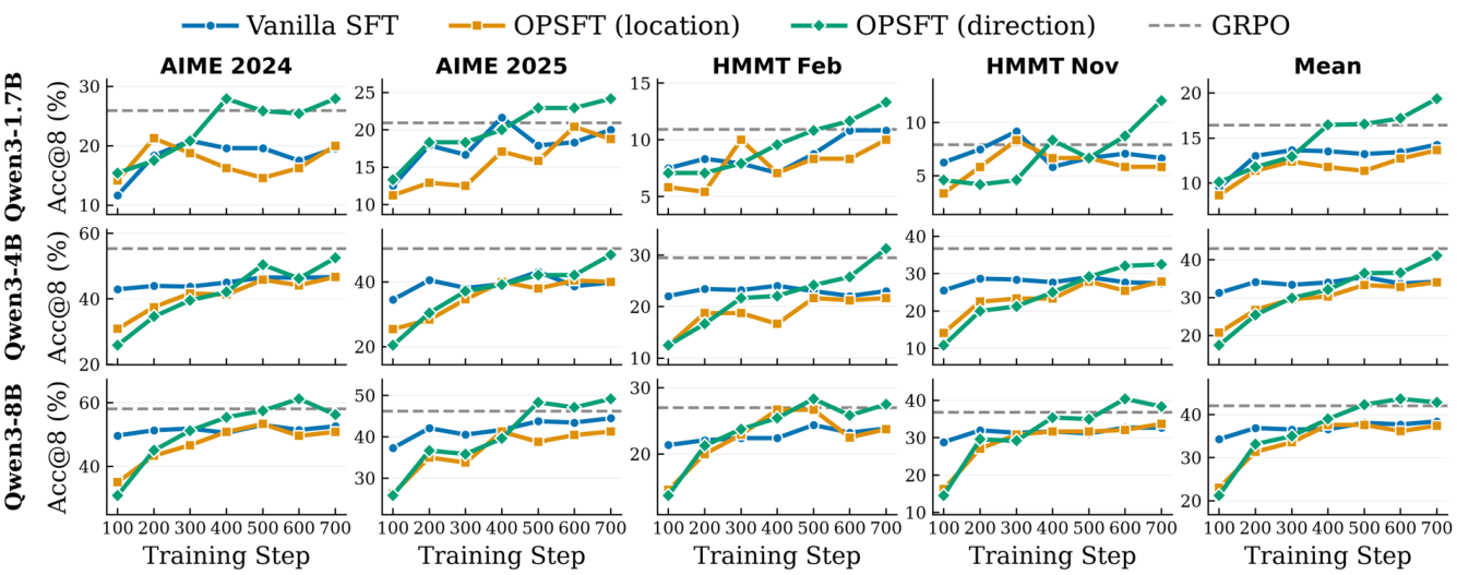
Figure 3 isolates the contribution: constraining SFT by location alone (which parameters) recovers only part of GRPO’s generalization, while constraining by direction closes nearly the entire gap and sometimes exceeds GRPO. This is the central empirical claim — the generalization-relevant on-policy information is in the sign structure, not just the support.
Quantitatively (Table 2, DeepMath training):
- DeepSeek-R1-Distill-LLaMA-8B: OPSFT reaches mean accuracy 26.56 in 8.1h, versus DFT at 19.90 in 14.1h and vanilla SFT trailing further behind. The direction-constrained variant uses 50 GRPO steps + 100 OPSFT steps against SFT/DFT’s 700 steps.
- Qwen3-8B: OPSFT achieves 41.67 mean accuracy in 8.9h, exceeding 100-step GRPO at 40.31 in 19.3h — i.e., >50% wall-clock reduction while improving generalization.
- The direction extracted from only 50 GRPO steps suffices to beat a 100-step GRPO run, suggesting the useful direction crystallizes very early in on-policy training.
- Code benchmarks (Table 5) replicate the pattern, indicating the effect is not math-specific.
The second application — applying OPSFT along the direction already traced out by a completed on-policy run, using fresh high-quality trajectories — continues to improve a GRPO-trained model without erasing on-policy gains, consistent with the view that the direction is the invariant to preserve.
Limitations and open questions
The paper uses sign-based direction constraints; whether a continuous-angle constraint (projection onto the cumulative-update subspace) would be strictly stronger is untested. The theoretical argument reduces on-policy updates to the advantage–score covariance but does not explain why its sign pattern generalizes better than SFT’s score-only direction — a mechanistic story (flat-minima selection, implicit regularization toward low-advantage-variance regions) is absent. The GRPO warm-up still requires rollouts and a reward model, so OPSFT does not eliminate on-policy infrastructure, only amortizes it. Finally, the stability of the extracted direction across datasets and seeds, and the scaling behavior at >8B, are not characterized.
Why this matters
If on-policy generalization is largely captured by a cheap-to-extract sign vector over parameters, then expensive RL post-training can be partially replaced by a short RL probe plus direction-constrained SFT, cutting post-training cost by half or more while matching or exceeding GRPO on standard benchmarks. It also reframes the SFT-vs-RL debate: the gap may be less about reward signal per se and more about which coordinate-wise sign pattern the optimizer commits to.
Source: https://arxiv.org/abs/2609.36659
PDE-JEPA: Predictive Representation Learning of Latent Dynamics Modeling for Parametric PDEs
Problem
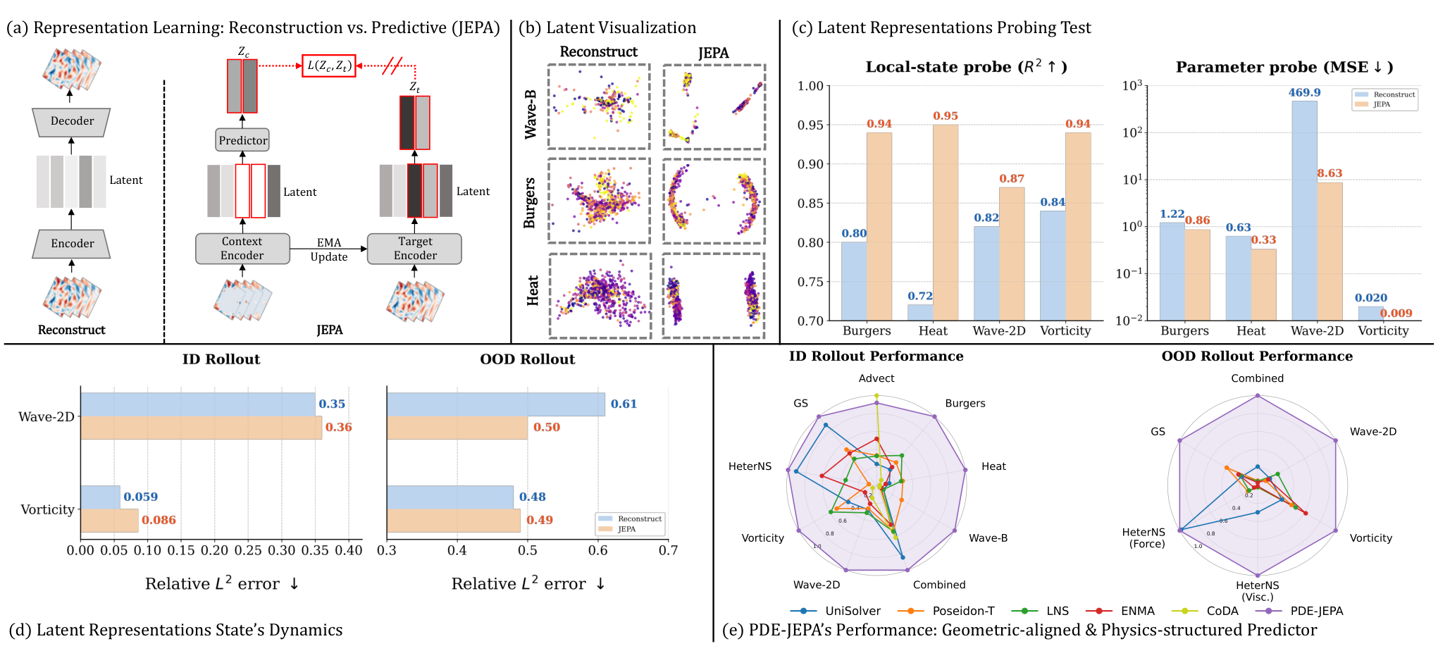
Neural surrogates for parametric PDEs are typically trained with reconstruction objectives: an encoder-decoder is driven to recover the physical fields \mathbf{u}_t, and dynamics are learned either in pixel space or in a reconstruction-aligned latent. The authors argue this biases the latent toward pointwise field recovery rather than toward the geometry of state evolution. They test the alternative: pretrain the encoder with a predictive (JEPA-style) objective — masked-latent prediction — and use the resulting space as the substrate for a dynamics learner. Their empirical observation is that JEPA features carry more physical information than MAE-style features (probing accuracy), yet directly rolling out a predictor on top of frozen JEPA features still gives mediocre forecasts. The gap between “informative” and “forecastable” motivates the method.
Method
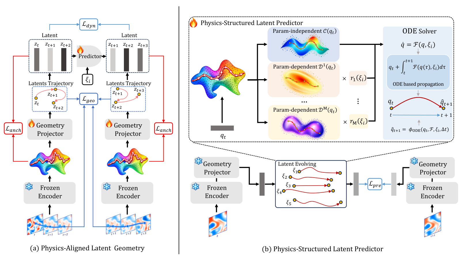
PDE-JEPA has three stages, with the encoder frozen after stage 1.
Stage 1 — Predictive pretraining. The encoder E is trained with JEPA-style masked-latent prediction on full trajectories, producing \mathbf{z}_{0:T}=E(\mathbf{u}_{0:T}),\quad \mathbf{u}_{0:T}\in\mathbb{R}^{|\mathcal{X}|\times T\times C},\ \mathbf{z}_{0:T}\in\mathbb{R}^{N\times T\times D}. For downstream use, states are re-encoded frame-wise so \mathbf{z}_t is causal. Importantly, the PDE parameter \bm{\xi} is withheld from both the encoder and the JEPA predictor during pretraining, pushing E toward parameter-agnostic features.
Stage 2 — Geometry projection. A lightweight projector g_\phi maps the frozen JEPA latents to a space in which latent trajectory geometry matches the geometry of physical evolution. Concretely, the alignment loss encourages pairwise distances/directions in the projected latent trajectory \{g_\phi(\mathbf{z}_t)\} to track those of \{\mathbf{u}_t\} over time. This is the step that turns an “informative” representation into a “dynamically consistent” one.
Stage 3 — Physics-structured latent predictor. On the aligned latent, the dynamics are decomposed into a parameter-independent evolution operator F_\theta and a parameter-dependent correction G_\psi(\cdot;\bm{\xi}), roughly \tilde{\mathbf{z}}_{t+1} = F_\theta(\tilde{\mathbf{z}}_t) + G_\psi(\tilde{\mathbf{z}}_t;\bm{\xi}), with \tilde{\mathbf{z}}_t = g_\phi(\mathbf{z}_t). The parameter branch is only introduced here, not in the encoder, so the shared operator F_\theta absorbs the common PDE physics while G_\psi carries parametric variation. Rollouts are performed in the aligned latent and decoded only for evaluation.
Results
Evaluation is on nine parametric PDE benchmarks: Advection, Burgers, Heat, Wave-B, Combined, Wave-2D, Vorticity (from Zebra), HeterNS (UniSolver), and Gray–Scott (ENMA), covering transport, diffusion, waves, reaction–diffusion, and 2D fluids. Metric is relative L^2 rollout error (ID split).
PDE-JEPA achieves the best or second-best on every benchmark. Representative numbers (lower is better):
- Burgers: 0.0428 vs. prior best 0.0869 (LE-PDE) — a 50.7% relative improvement.
- Heat: 0.0274 vs. 0.0933 (Poseidon-T) — 70.6%.
- Wave-B: 0.0350 vs. 0.1093 (Poseidon-T) — 68.0%.
- Wave-2D: 0.1140 vs. 0.2070 (Zebra) — 44.9%.
- Vorticity: 0.0348 vs. 0.0592 (LNS) — 41.2%.
- Combined: 0.0074 vs. 0.0085 (CAPE) — 12.9%.
- HeterNS: 0.0089 vs. 0.0098 (UniSolver) — 9.2%.
- Gray–Scott: 0.0284 vs. 0.0323 (UniSolver) — 12.1%.
- Advection: 0.0074 vs. 0.0068 (CoDA) — the one setting where PDE-JEPA is second (−8.8%).
Notably, PDE-JEPA outperforms foundation-model surrogates (UniSolver, MPP, DPOT-S, Poseidon-T), in-context solvers (Zebra, ViT variants), and reconstruction-based latent solvers (LE-PDE, LNS, MAE-PDE, ENMA) despite using a frozen encoder plus two lightweight modules.
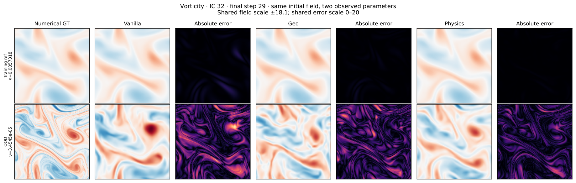
The Vorticity case study isolates the contribution of each stage: a vanilla JEPA + predictor baseline has visible error structure on the final timestep; adding geometry alignment reduces coherent large-scale error, and the physics-structured predictor further suppresses parameter-dependent residuals.
Limitations and open questions
The encoder is frozen after Stage 1; whether end-to-end fine-tuning with the geometry/physics objectives would help or destabilize training is untested. The geometry projector depends on a notion of “physical evolution geometry,” which the paper operationalizes via trajectory distances — it is unclear how this behaves for shock-dominated or discontinuous solutions, where field-space geometry is non-smooth. Reported numbers are ID rollouts; OOD-parameter extrapolation is claimed in the overview figure but not quantified in the shown table. Finally, the parameter-independent/dependent decomposition assumes the family’s physics is dominated by a shared operator — a reasonable assumption for the nine benchmarks here, but likely strained for multi-physics mixtures.
Why this matters
The result is a concrete demonstration that predictive (JEPA-style) pretraining can outperform reconstruction pretraining for PDE surrogates, provided the latent is subsequently aligned to the geometry of state evolution. The two-stage recipe — align geometry, then factor dynamics into shared + parametric components — is simple, modular, and portable to other operator-learning settings.
Source: https://arxiv.org/abs/2609.34715
FrameMorrow: Future-guided Frame Selection with Prospective Tokens for Long-Horizon Video Generation
Problem
Autoregressive long-horizon video generators accumulate history faster than they can attend to it. Dense attention over all past frames is quadratic and quickly becomes infeasible past the one-minute mark, while naive truncation discards content that may matter many seconds later (a character’s clothing, the layout of a room, an object that leaves and re-enters). Existing retrieval-style approaches (e.g., LongLive-RAG) score history by similarity to the current context. The authors argue this is the wrong objective: features relevant to the present view may be redundant with the recent context buffer, while features relevant to what will be generated next may look dissimilar to the present but are precisely what the backbone needs.
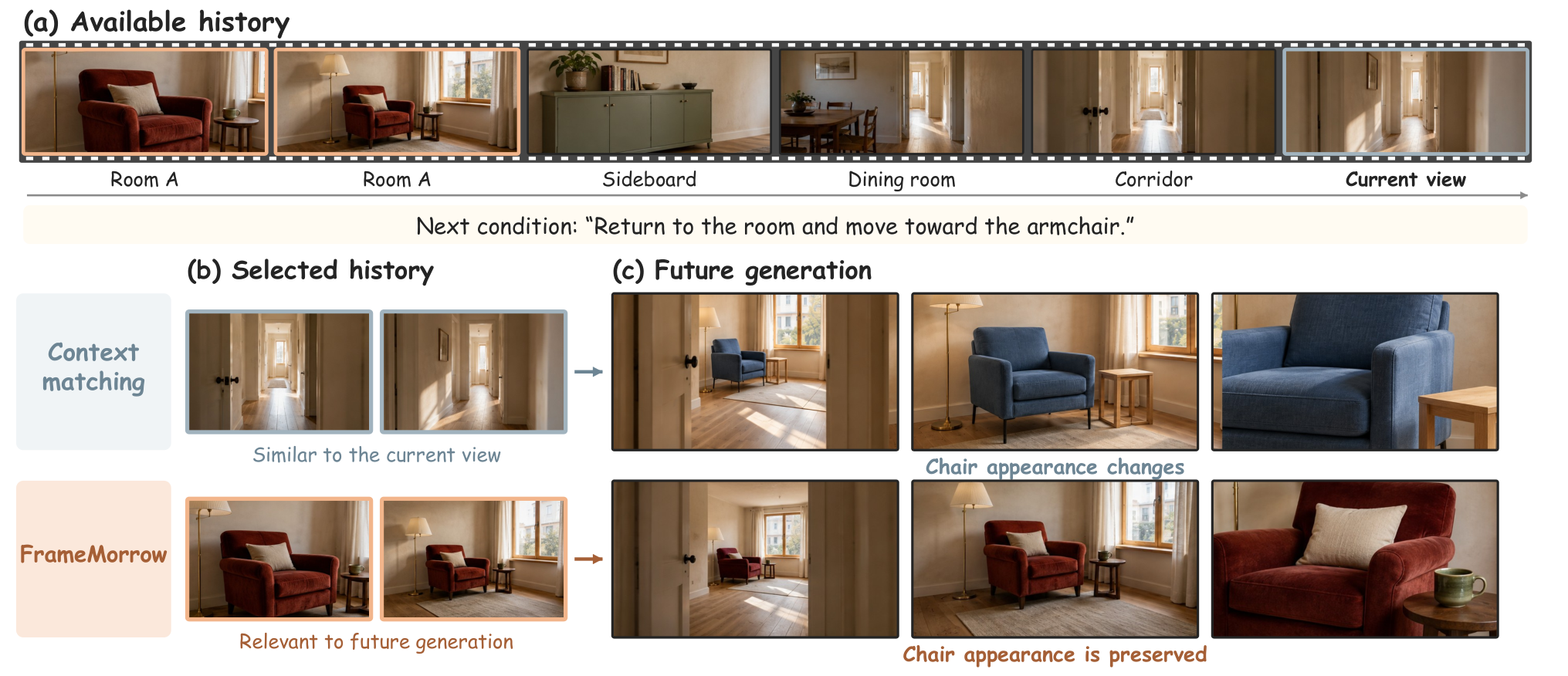
The problem matters because interactive and world-model settings explicitly make the future condition c_t^+ (a prompt continuation, an action, a camera motion) available before the next chunk is rolled out, and this signal is currently underused for memory management.
Method
At rollout step t, let the recent context be \mathcal{L}_t = \{x_{t-L+1}, \ldots, x_t\} and the eligible long-term history be \mathcal{H}_t = \{x_{\tau_i}\}_{i=1}^N with \tau_i \le t - L. \mathcal{L}_t is observed by the selector but not eligible for retrieval, so it informs what to recall without competing for the memory budget K.
A selector S_\theta emits M prospective tokens from (\mathcal{H}_t, \mathcal{L}_t, c_t^+). These tokens are learned queries intended to represent the information needs of the upcoming chunk — crucially, without decoding the chunk itself. They produce per-frame relevance scores:
\hat{\mathbf{r}}_t = S_\theta(\mathcal{H}_t, \mathcal{L}_t, c_t^+) \in \mathbb{R}^N, \quad \mathcal{I}_t = \mathrm{TopK}(\hat{\mathbf{r}}_t, K), \quad \mathcal{M}_t = \mathcal{H}_t[\mathcal{I}_t].
Selected frames are timestamp-ordered and fed through the frozen backbone’s native conditioning interface. Default settings are K=4 and M=4.
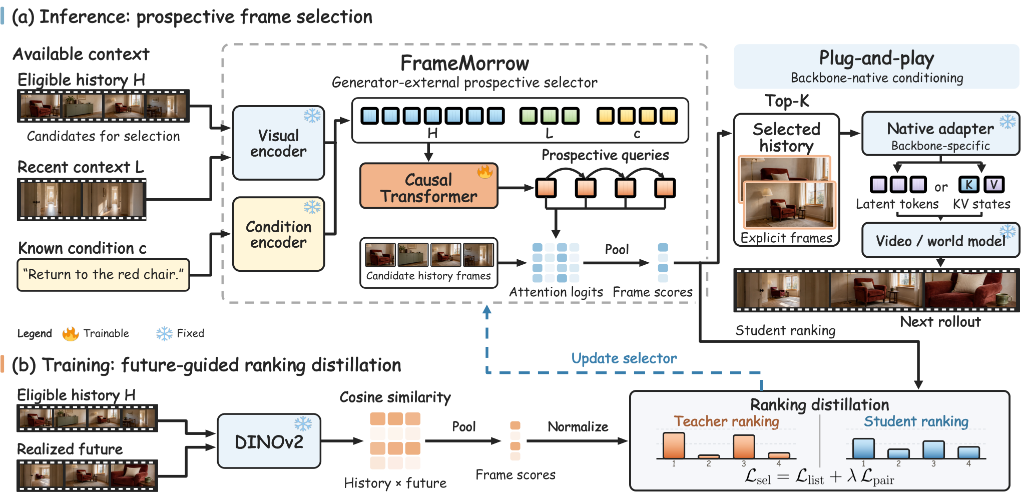
Supervision is the interesting piece. During training, the realized future chunk is available. A frozen DINOv2 teacher computes similarity between each eligible historical frame and the realized future, producing a ranking over \mathcal{H}_t. The prospective tokens are trained so that \hat{\mathbf{r}}_t matches this future-grounded ranking. At inference the future is unobserved, but the tokens have learned to predict which historical frames will be visually relevant from (\mathcal{H}_t, \mathcal{L}_t, c_t^+) alone. Because the output is explicit frames rather than KV-cache slices or hidden states, the module is plug-and-play across heterogeneous backbones (Self-Forcing, LongLive, Causal Forcing, CausVid, ShotStream, Matrix-Game 3.0, WorldMem, and closed-source Seedance/Kling via reference-image interfaces).
Training uses 10K OpenVidHD videos reorganized into streaming prompts for text-conditioned generation, and 10K chunk-aligned Sekai Game-Walking segments with pseudo-actions from camera motion for action-conditioned world models.
Results
The 60-second interactive video table shows consistent gains across every backbone pair. The largest absolute improvements come where the base model is weakest in long-horizon consistency:
- Self-Forcing: quality 78.71 → 81.74, consistency 84.95 → 89.30, aesthetic 58.16 → 60.62. Segment-wise CLIP average: 26.39 → 28.05, with the biggest gains in the 30–60s window (e.g., 40–50s: 23.37 → 26.60).
- Causal Forcing: quality 76.00 → 78.66, consistency 80.46 → 83.48, CLIP avg 24.53 → 25.24.
- LongLive 1.0 (already strong): quality 83.49 → 84.06, consistency 92.62 → 93.21, CLIP avg 28.75 → 29.08.
- CausVid: CLIP avg 28.63 → 29.03, with monotonic improvement across all six 10-second windows.
Multi-shot results follow the same pattern: ShotStream jumps on consistency 92.75 → 96.76 and quality 83.12 → 84.85, though aesthetic drops slightly (62.30 → 61.74). LongLive 2.0 shows smaller but uniform gains.
The decay profile is informative: for Self-Forcing, segment CLIP drops from 30.40 (0–10s) to 23.02 (50–60s) without FrameMorrow, a 7.4-point degradation; with FrameMorrow the drop is 30.56 → 26.01, roughly halving the long-horizon collapse. This is consistent with the hypothesis that current-context matching retains redundant frames while losing semantically important history.
Limitations and open questions
- The ranking teacher is DINOv2, which encodes appearance well but is weak on motion and action semantics. For world-model experiments, this likely bottlenecks action-aligned retrieval, though the paper reports Qwen3-VL-based action alignment as the downstream metric rather than directly validating the teacher.
- K=4 frames is small; results do not characterize how performance scales with K, or whether token count M needs to grow for scenes with multiple independent entities.
- Supervision requires realized futures, so pure online or self-play world-model training is not addressed.
- The method inherits each backbone’s reference-conditioning quirks; the ShotStream aesthetic regression suggests selected frames can occasionally conflict with the backbone’s own aesthetic prior.
- No wall-clock comparison against \infty-RoPE or Deep Forcing is excerpted; the cost of running the selector at every rollout step relative to the KV savings is not quantified in the shown sections.
Why this matters
Framing long-video memory as predicting future information needs rather than matching the present is a clean reformulation that cleanly decouples retrieval from the backbone, and the empirical gains — particularly the halved consistency decay on Self-Forcing past 30 seconds — suggest the current-context-matching baseline in long-horizon generation has been leaving substantial headroom on the table.
Source: https://arxiv.org/abs/2609.38839
World Action Modeling with Progressive Visual Planning
Problem
World action models (WAMs) couple visuomotor policy learning with future-frame prediction: the model is trained to jointly roll out video and action chunks from an initial image and language instruction, so that visual dynamics prediction regularizes and conditions action generation. The practical bottleneck is long-horizon control. Dense video rollouts are expensive at inference (diffusion video generators require many denoising steps over tens of frames), while the recent shortcut of predicting only a single final goal frame (FGP) tells the policy where the episode ends but not how to interpolate between the current state and that terminus. Both failure modes hurt long-horizon tasks where sub-skills (approach, grasp, transport, place) must be anchored to intermediate visual states.
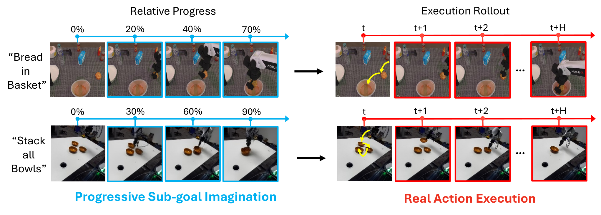
ProWAM targets this gap by replacing dense-video prediction and single-frame FGP with a sparse, ordered sequence of visual sub-goals indexed by relative task progress \tau \in (0,1], co-generated with action chunks by a shared video backbone.
Method
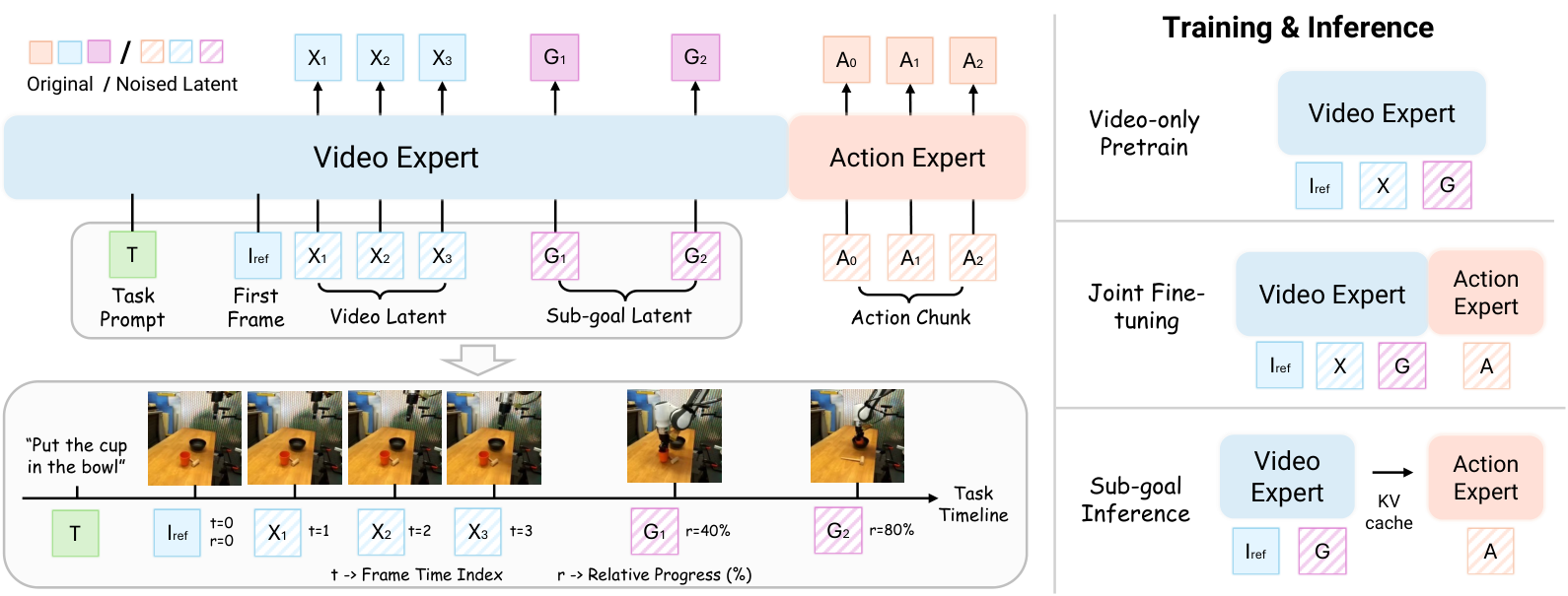
ProWAM factorizes a WAM into a video expert and an action expert sharing the Wan2.2-TI2V-5B video backbone. Given instruction \mathbf{T} and reference frame \mathbf{I}_{\mathrm{ref}}, the model jointly denoises three latent streams:
- future-video latents \mathbf{X} (used only during pretraining as a visual-dynamics objective),
- progressive sub-goal latents \mathbf{G} = \{g_{\tau_1}, \ldots, g_{\tau_k}\} at k selected relative progress positions \tau_i,
- action chunk latents \mathbf{A} aligned to the segments between consecutive sub-goals.
The sub-goals generalize FGP: FGP is the special case k{=}1,\ \tau_1{=}1. During training, sub-goal positions are sampled so that each g_{\tau_i} supervises the visual state the robot should reach after a specified fraction of the episode.
Training proceeds in two stages:
- Video-only pretraining. The video expert is trained on large-scale action-free robot and egocentric video to predict both dense future frames and the progressive sub-goal sequence. This exploits the scale asymmetry between action-free video and robot demonstrations: sub-goal planning is learned mostly from the former, offloading visual planning from the action policy.
- Joint fine-tuning. On robot demonstrations, the action expert is trained with a diffusion/flow-matching action objective conditioned on sub-goal features from the video expert. The video branch keeps sub-goal prediction as a co-training objective so the shared representation stays sub-goal-aware.
The key inference-time optimization is caching. Instead of iteratively denoising a full video rollout at every replan, ProWAM runs a single forward pass of the video expert to produce sparse sub-goal KV features \{K_{\tau_i}, V_{\tau_i}\}. The action expert then cross-attends to this cached set during its (lightweight) action denoising. On replanning, only the action expert needs to rerun unless the sub-goal cache is refreshed. This decouples control-rate action denoising from the heavy video-expert evaluation and avoids the dense-rollout cost that bottlenecks prior WAMs.
Two variants isolate the role of the visual prior: ProWAM-Base initializes from the Wan2.2-TI2V-5B base without Stage-1, and ProWAM uses the Stage-1 pretrained video expert.
Results
ProWAM is evaluated on LIBERO and LIBERO-Plus, RoboTwin, RoboCasa365, and zero-shot Franka deployments, following the protocols of concurrent WAM work (Black et al., 2025; Bu et al., 2025b; Yuan et al., 2026; Luo et al., 2026a). The reported headline is superior out-of-distribution robustness across these benchmarks, with the sub-goal-conditioned variant improving over FGP baselines and dense-video WAMs; the pilot study in the appendix also confirms that self-generated final goals already improve baselines in most settings, so the gains from progressive sub-goals are measured on top of a strong FGP control. (The excerpt provided does not enumerate per-benchmark success rates, so I refer the reader to Section 4 and the appendix for the full tables.)
The architecture choice is validated on compute as well: because inference uses one video-expert pass to cache sparse \mathbf{G} features and then only action denoising at control rate, per-step latency is dominated by the action expert rather than video generation—removing the iterative full-video rollout cost that limited earlier WAMs.
Failure modes
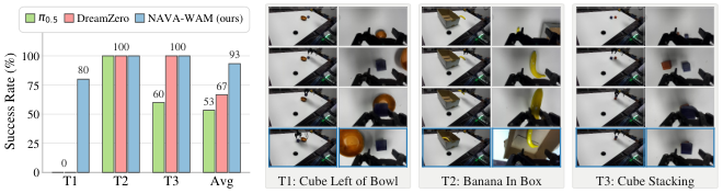
A qualitative failure on “Cube Stacking” illustrates the dependence on sub-goal fidelity: when the predicted sub-goal has ambiguous contact geometry, the policy opens the gripper prematurely.
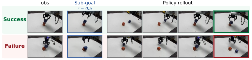
This exposes the central weakness of the design: ProWAM’s action policy is as good as its sub-goals, so sub-goal hallucination—especially for fine-grained contact-rich interactions where pixel-level ambiguity hides geometric constraints—translates directly into execution errors. Open questions include: (i) how to inject explicit geometric/contact priors into sub-goal generation; (ii) whether online sub-goal re-selection (dynamic \tau schedules) outperforms a fixed sparse set; (iii) how sub-goal cardinality k should scale with task horizon; and (iv) whether the sub-goal cache can be partially refreshed to correct drift without triggering a full video-expert pass.
Why this matters
ProWAM is a clean statement of a design principle for WAMs: generate a sparse, ordered visual plan and condition actions on cached features from it, instead of either (a) generating dense video rollouts you throw away or (b) predicting a terminal goal that underspecifies the trajectory. Combined with action-free video pretraining of the planner, this is a plausible route to scaling visuomotor policies to long horizons without paying video-generation cost at control time.
Source: https://arxiv.org/abs/2610.02508
Native Action-Prior Learning from Videos for World Action Models
Problem
World action models (WAMs) couple future-video prediction with action prediction, giving the policy a dynamics-aware prior. The bottleneck is action-labeled trajectories: robot teleop data is scarce, while observation-only video is abundant. The two dominant ways of exploiting unlabeled video are both indirect. Vision-representation pretraining (e.g., MAE/VideoMAE-style encoders) yields features that must be re-fitted to control. Latent-action learning (LAPO, DynaMo, CoMo) infers a latent action \hat{a}_t from (z_{t-1}, z_t) and uses it as surrogate supervision, but the latent space is not calibrated to any embodiment and requires a separate grounding step.
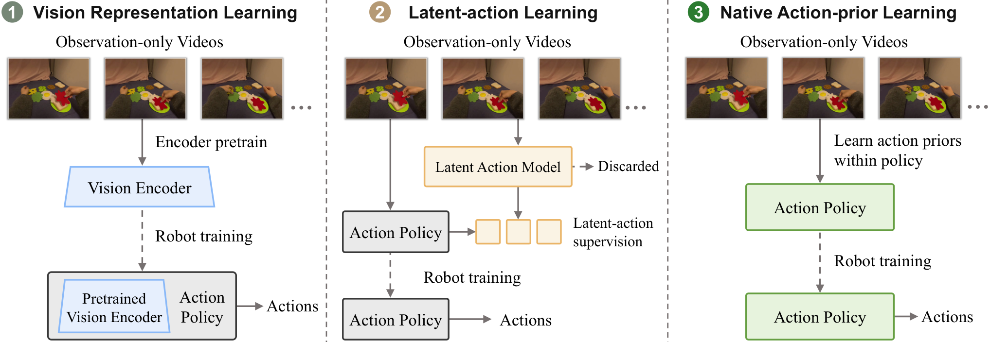
NAVA-WAM proposes a third option: pretrain the action module itself directly on observation-only video, with no intermediate representation or latent action interface.
Method
The policy \mathcal{P}_\theta(a_{t:t+H-1}\mid o_t, l, q_t) predicts a continuous H-step chunk in \mathbb{R}^{H\times d_a}. Two streams are instantiated as DiTs: a Video-DiT initialized from Wan2.2-5B, and a 1B-parameter Action-DiT (hidden dim 1024). A frozen spatiotemporal VAE E encodes o_{0:T} into latents z_{0:K}, so each (z_{k-1}, z_k) is a visual transition.
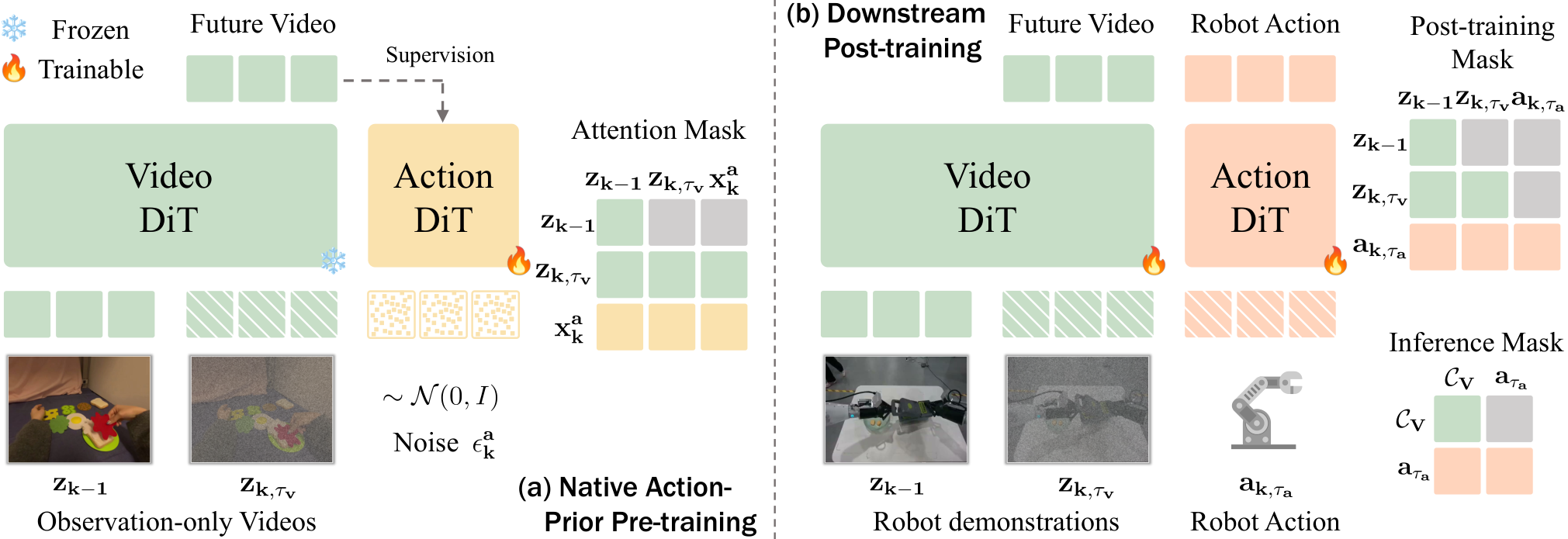
Stage 1 — Native action-prior pretraining (\mathcal{D}_v). Only the Video-DiT receives a flow-matching loss on future-video latents. Crucially, gradients reach the Action-DiT through a transition-structured joint attention that pairs each video transition (z_{k-1}, z_k) with an action token slot. Because future-video prediction is causally determined by the (implicit) action, optimizing the shared attention forces the Action-DiT tokens to encode the quantity most predictive of the transition — an action-relevant prior — without ever instantiating a latent-action vocabulary.
Stage 2 — Joint post-training (\mathcal{D}_r). Both streams are trained with video and action flow-matching losses, weighted \lambda_v = \lambda_a = 1. An asymmetric attention pattern decouples the visual branch from the iterative action denoiser: visual tokens attend only once, while action tokens iterate across denoising steps. This means that at inference, the video stream can be dropped entirely and only action tokens are denoised — closed-loop control without rolling out future frames.
Results
LIBERO / LIBERO-Plus. NAVA-WAM reaches 99.0% ID / 83.5% OOD, matching Being-H0.7 (99.2 / 82.1) and Image-WAM (98.4 / 83.1), and substantially above latent-action-centric WAMs such as JEPA-VLA (96.4 / 25.6) and Fast-WAM (97.6 / 51.5). The OOD gap is the more informative signal: approaches that rely on indirect transfer collapse under LIBERO-Plus distribution shifts.
RoboTwin 2.0. Training only on 50 Clean demos per task, NAVA-WAM scores 88.5% Clean and 73.6% Random. The Random (OOD) number is the headline: the previous best, MV-WAM, achieves 55.7%, and Image-WAM only 37.6%. Standard direct policies (\pi_0, UP-VLA, DP, RDT) are below 17% in Random. This is a 17.9-point absolute OOD improvement over the strongest WAM baseline.
Real robot (Franka FR3, DROID post-training, no task-specific finetuning). Across three tabletop tasks with five trials each, NAVA-WAM achieves 93.3% average success. On T1 (a spatial-relation task), \pi_{0.5} and DreamZero-DROID fail all trials; NAVA-WAM succeeds.
Ablations. The pretraining-vs-label-budget sweep on RoboTwin 2.0 Random is the most direct test of the paper’s claim:
| Demos/task | None | Repr. | Latent-action | NAVA |
|---|---|---|---|---|
| 10 | 60.5 | 58.2 | 61.6 | 66.5 |
| 25 | 67.6 | 60.6 | 65.0 | 72.0 |
| 50 | 69.7 | 68.1 | 71.2 | 73.6 |
Representation-based pretraining actually hurts at 10 and 25 demos — consistent with the “indirect transfer” critique. The action-relevance probe (ridge regression R^2 from frozen features to ground-truth actions) further supports the mechanism: representation features saturate at R^2 = 0.153 with 100% probe data, CoMo latent actions at 0.203, while NAVA features score higher (full table in the paper), indicating the pretrained Action-DiT tokens are more linearly predictive of true robot actions than either alternative.
Limitations and open questions
- The Video-DiT is initialized from Wan2.2-5B; it is unclear how much of the OOD gain is attributable to that generative prior vs. the native action-prior scheme. The ablation isolates pretraining data but not initialization.
- Pretraining data (Open X-Embodiment, AgiBotWorld, EgoDex) is still robot/egocentric manipulation video. The claim that observation-only video suffices has not been tested on fully in-the-wild internet video, where visual distribution shifts are much larger and no proprioception is correlated.
- The transition-structured joint attention assumes a one-to-one mapping between visual transitions and action slots at the VAE’s temporal rate; mismatches between VAE stride and policy horizon H are not analyzed.
- Only a 1B Action-DiT is reported. Scaling behavior of the native prior with Action-DiT size is open.
Why this matters
NAVA-WAM is a clean demonstration that the “observation-only video \to policy” pipeline does not need an intermediate interface — neither a reusable visual encoder nor a latent-action codebook. Gradients from future-frame prediction, routed through a shared attention topology, suffice to pretrain the action head itself, and the resulting policy generalizes markedly better OOD (73.6% vs. 55.7% on RoboTwin Random; 93.3% on a zero-shot Franka deployment).
Source: https://arxiv.org/abs/2610.03391
Hacker News Signals
Run Qwen 3.8 Flash Next (125B) on consumer hardware (RTX 4090) at 100T/s
Strata is a custom inference runtime targeting single-consumer-GPU deployment of large models that would normally require multi-GPU server setups. The headline claim is 100 tokens/s for a 125B-parameter model on a single RTX 4090 (24 GB VRAM). Achieving this requires aggressive quantization (likely 2–3 bit effective weight precision), speculative decoding with a draft model, and careful KV-cache management to fit within VRAM constraints. The repo combines CUDA kernels optimized for the 4090’s architecture (Ada Lovelace, FP8 tensor cores) with CPU offloading that hides transfer latency behind compute. The key engineering challenge at this scale is keeping the GPU saturated despite the memory bandwidth bottleneck: a 125B model even at 4-bit requires ~62 GB, so the runtime tiles weights across VRAM and system RAM, prefetching the next layer while the current one executes. Speculative decoding with a small draft (possibly a 1–3B model that fits entirely in VRAM) generates candidate token sequences that the full model verifies in parallel, multiplying effective throughput. The 100 T/s figure is almost certainly measured on short-context generation with a warm cache; long-context performance with large KV caches degrades substantially as offloading bandwidth becomes the bottleneck. The project is early-stage and the quantization quality relative to BF16 baseline is not benchmarked in the repo, which is the main open question for practical use. Community skepticism in the thread focuses on whether perplexity degradation at such aggressive quantization levels makes the output useful for non-trivial tasks.
From the creator of Redis: run LLM locally with ds4
Salvatore Sanfilippo (antirez) has released ds4 (Dwarf Star 4), a minimal local LLM runtime written to prioritize simplicity and hackability over performance. The design philosophy mirrors his Redis aesthetic: a small, auditable C codebase that does one thing — load GGUF-format models and run autoregressive inference — without the abstraction layers of llama.cpp or llm.c. The implementation handles transformer inference manually, supporting the standard multi-head attention with RoPE positional encoding and RMS-norm, in a few thousand lines. It targets developers who want to understand or modify the inference stack rather than users wanting maximum throughput. GGUF support means it interoperates with the large ecosystem of quantized model weights already published for llama.cpp. The interesting engineering choice is forgoing batching and many inference optimizations entirely to keep the code readable. Memory layout follows the GGUF tensor ordering directly to avoid a separate loading pass. Sanfilippo has written accompanying blog posts explaining each component, making it a credible learning resource. Practical throughput is lower than llama.cpp, but for single-user interactive use on CPU the difference is tolerable on modern hardware. The HN discussion centers on the value of “readable” implementations versus optimized ones, with particular interest in whether the codebase could serve as a teaching tool for graduate ML systems courses. The main limitation is the lack of GPU support at launch; it runs on CPU only, so 70B+ models are impractical.
Source: https://dwarfstar.sh/
Greg Kroah-Hartman: Security in the LLM Age
Kroah-Hartman’s talk addresses a concrete systems security concern: the Linux kernel development pipeline increasingly intersects with LLM-generated or LLM-assisted code contributions, and the existing review infrastructure was not designed with that threat model in mind. His core argument is that LLMs lower the cost of generating plausible-looking but subtly incorrect or malicious patches to near-zero, which shifts the attacker economics for supply-chain attacks on the kernel. The existing defense is human review, but review bandwidth is finite and reviewers exhibit automation bias when patches look stylistically correct. He discusses specific mitigations: stricter identity verification for new contributors, automated static analysis gates that catch a broader class of issues before human review, and skepticism toward patches that touch security-critical subsystems from accounts with shallow history. He is careful to distinguish LLM-generated bugs (accidental, from developers using code assistants uncritically) from LLM-generated attacks (deliberate), noting the defenses differ. The XZ utils backdoor is referenced as a precedent for slow, patient supply-chain infiltration; LLMs potentially accelerate the “fake contributor building credibility” phase. The talk does not propose new cryptographic or formal-verification solutions but argues for process hardening: smaller trusted maintainer groups for sensitive subsystems, more conservative patch acceptance criteria, and better tooling to surface statistical anomalies in contribution patterns. For kernel developers and open-source maintainers more broadly, the practical takeaway is that social engineering surface area has expanded significantly.
GPT-Synopsys: Frontier Intelligence to Revolutionize Chip Design
OpenAI and Synopsys have announced a joint product integrating frontier LLMs into the Synopsys EDA toolchain. The technical substance, as far as disclosed, covers three areas: natural-language RTL generation and modification within the Design Compiler/Fusion Compiler flows, AI-assisted timing closure and floorplanning suggestions, and automated testbench generation with coverage-directed feedback. The RTL generation component is the most technically interesting: rather than treating it as pure code generation, the system is framed as operating within the constraint space of synthesis targets (area, power, timing), using the LLM to propose microarchitectural alternatives that a downstream synthesis tool then evaluates. This closes the loop that pure LLM code generation misses — the model cannot intrinsically reason about post-synthesis QoR, but constrained search guided by LLM proposals can. Timing closure assistance involves the model suggesting placement and routing directives based on violation reports, which is currently a highly manual expert task. The main skepticism in the HN thread is around whether this is meaningful AI integration or a UI layer over existing Synopsys AI features (which already exist in tools like DSO.ai). The announcement lacks benchmark numbers comparing AI-assisted versus manual flows on representative designs. Chip design cycles are long enough that external validation will lag by months to years. The deeper question is whether frontier LLMs trained on general code have enough coverage of Verilog/SystemVerilog idioms and synthesis semantics to be useful without extensive domain-specific fine-tuning.
Show HN: AI search for every photo and every frame of video on macOS
SCM (Screen Content Manager) is an open-source macOS tool that indexes screenshots, photos, and video frames using a local CLIP-based embedding pipeline, storing vectors in a local database for natural-language and image-similarity search. The technical pipeline: periodic screen capture or manual import feeds frames into a CLIP vision encoder running via Core ML on the Neural Engine, generating 512- or 768-dimensional embeddings that are stored in a local vector store (SQLite with custom vector indexing or FAISS, per the repo). Query time involves encoding the text query with CLIP’s text encoder and performing approximate nearest-neighbor search. Running CLIP inference on the Apple Neural Engine rather than CPU gives roughly 5–10x throughput improvement for batch indexing. The privacy-first design (everything local, no cloud API calls) is the stated differentiator from cloud-based alternatives. The main engineering challenges are: (1) deduplication across near-identical frames, handled with perceptual hashing before CLIP inference to avoid redundant embeddings; (2) index size management as the corpus grows, addressed with configurable retention windows; (3) incremental indexing to avoid re-processing the entire archive on each run. CLIP’s known weaknesses apply — fine-grained text in images, specific faces, and precise object counting are unreliable. The repo is early and the ANN index implementation is basic; scaling to millions of frames would require more sophisticated indexing. HN discussion focuses on the privacy angle and comparison to Apple’s own on-device search capabilities introduced in recent macOS versions.
Source: https://github.com/allenv0/SCM
Getting the most out of Opus 5.5 in Claude and Claude Code
Anthropic’s engineering blog post describes practical prompt-engineering and agentic-loop design patterns specific to Claude Opus 5.5, with particular focus on Claude Code (the agentic coding assistant). The technically substantive claims: Opus 5.5 has a 200K token context window, and the post details how to structure long contexts so that critical instructions survive the known middle-of-context attention degradation. Recommendations include placing constraints and success criteria at both the start and end of the prompt rather than the middle, and using explicit XML-tagged sections (<instructions>, <constraints>) that the model has been trained to weight more heavily. For agentic loops, the post advises against over-decomposing tasks into many small tool calls, noting that Opus 5.5 can maintain coherent multi-step plans within a single context and that excessive scaffolding overhead degrades performance. There is guidance on structured output: using JSON schema enforcement via the API’s response_format parameter reduces parse errors significantly versus free-form generation. For Claude Code specifically, the post describes how to write CLAUDE.md files that persist project context across sessions, recommending they contain architectural invariants rather than ephemeral state. The post also acknowledges that Opus 5.5 sometimes over-explains; the suggested mitigation is explicit instruction to skip reasoning preamble. The HN discussion is a mix of practitioners sharing what actually works and skeptics noting that model-specific prompt guides become stale quickly. The lack of ablation data for the recommendations is a consistent criticism.
Source: https://claude.dev/blog/getting-the-most-out-of-opus-5-5/
We ported the original Doom to SQL
CedarDB implemented a fully playable Doom engine in SQL, targeting their own analytical database system. The technical core is that the entire game loop — BSP tree traversal for visibility, raycasting, sprite rendering, game state updates — is expressed as a sequence of SQL queries executed each frame. CedarDB’s query engine is fast enough on in-memory tables to sustain interactive frame rates. The most interesting engineering problem is expressing mutable game state in a language designed for set operations on immutable relations. The solution uses temporary tables and UPDATE/DELETE statements to represent the game world, with the renderer implemented as a chain of CTEs that walk the BSP tree and compute which wall segments are visible from the player’s position. The raycasting pass is a recursive CTE that traces rays across sectors. Sprite ordering uses a window function over depth-sorted entities. The BSP tree itself is stored as a table with parent/child foreign keys, and tree traversal is a standard recursive CTE pattern. Input handling bridges C event polling to SQL parameter injection per frame. This is primarily a demonstration of CedarDB’s query throughput on complex, iterative workloads — BSP traversal is not a natural SQL workload, and achieving playable performance validates the engine’s efficiency on recursive and join-heavy queries. The blog post provides detailed query examples. The HN thread is almost uniformly positive, focusing on the recursive CTE implementation of tree traversal and what it implies about the database’s optimizer.
Show HN: Made an open-source Lego AI generator
ldraw-nova generates LDraw-format Lego model files from text or image prompts using a combination of an LLM for high-level structure planning and a constrained generation layer that enforces LDraw part validity. The LDraw format represents models as lists of part placements: each line specifies a part ID, transformation matrix, and color. The constraint problem is non-trivial — valid Lego models must satisfy physical connectivity rules (studs align to anti-studs on a 20 LDU grid), and the part catalog has thousands of valid IDs with irregular geometries. The generation approach: the LLM produces a coarse structural description (e.g., “4x2 brick at position X connects to 2x2 plate at Y”), and a post-processing layer snaps coordinates to the LDraw grid and resolves part IDs against the official catalog. This is similar in spirit to constrained decoding but implemented as a post-hoc correction step rather than token-level constraints. The system uses BrickLink’s part database for ID resolution and LDView or LDraw-compatible renderers for visualization. The main failure mode is physically invalid assemblies: the LLM-generated placements sometimes violate connectivity constraints in ways the snapping layer cannot recover from, resulting in floating bricks or interpenetration. The repo is open-source and uses the Python LDraw library for file I/O. HN discussion covers the difficulty of spatial reasoning for LLMs and whether a specialized constraint solver (CSP or SAT-based) over the stud connection graph would outperform the LLM-then-correct approach.
Noteworthy New Repositories
bilibili/Index-Translate
A multilingual neural machine translation model family released by Bilibili. The project targets high-quality translation across a broad set of language pairs, likely built on a large transformer seq2seq backbone fine-tuned for translation-specific tasks. The release follows the trend of large Chinese internet companies open-sourcing production-grade NLP infrastructure rather than purely academic demos. For practitioners, the value is in having a model family — multiple size tiers — allowing deployment tradeoffs between latency and quality. The clean-room origin from a company running bilingual (Chinese/Japanese/English) content at scale suggests the training data distribution is more representative of real web and subtitle content than academic corpora. Key questions for adoption: tokenizer coverage for low-resource languages, quantization support for inference, and whether the license permits commercial use. Worth evaluating head-to-head against NLLB-200 and Opus-MT on domain-specific benchmarks.
Source: https://github.com/bilibili/Index-Translate
storytold/photocraft
A clean-room reimplementation of Adobe Photoshop written in pure Rust. Clean-room means the implementation is derived from observed behavior and public specifications rather than decompiled or licensed Adobe code, which matters for the legal standing of any derivative work. The Rust choice gives memory safety without a GC, which is critical for image buffer manipulation at scale — raster operations on large canvases can involve gigabytes of heap-allocated pixel data where GC pauses would be visible. The core technical challenge is implementing a compositing engine with correct layer blend modes (Porter-Duff operators, the full set of CSS/PDF blend modes), a non-destructive adjustment layer pipeline, and selection/masking infrastructure. It is currently early-stage, and feature parity with Photoshop is a multi-year target. The most immediate comparison is Graphite (also Rust-based), though Graphite leans vector-first. Useful as a reference for Rust GUI architecture and image processing pipeline design regardless of completeness.
Source: https://github.com/storytold/photocraft
LockedinLabs-AI/agent-console
Local-first observability dashboard for AI coding agents — specifically Claude Code and OpenAI Codex sessions. Tracks per-session token counts, cache hit/miss rates, model selections, and cost attribution entirely on-device, with an optional self-hosted team hub for aggregating data across machines. The architecture avoids sending telemetry to a third-party SaaS, which is the main differentiator against hosted dashboards. Policy hooks allow attaching pre/post-call logic — useful for enforcing spend limits or logging prompts for audit. The macOS binary is Apple-signed and notarized, and releases carry attestations, which matters for enterprise security review. The “presenting mode” feature suggests a UI for sharing session state in demos or pair-programming contexts without exposing sensitive API keys. For teams running agentic coding workflows at volume, the cost attribution layer alone justifies adoption — multi-agent sessions can produce surprising token counts that are invisible without instrumentation. MIT licensed.
Source: https://github.com/LockedinLabs-AI/agent-console
storytold/filmcraft
Clean-room Rust reimplementation of Adobe Premiere Pro — a non-linear video editor (NLE). This is technically the most demanding of the storytold suite: an NLE must handle heterogeneous media (multiple codecs, frame rates, sample rates), a timeline engine with frame-accurate seeking, real-time compositing for previews, and an audio mixing graph. In Rust, the codec layer would naturally wrap FFmpeg via ffmpeg-next or similar bindings, though a clean-room claim would require careful scoping of what “clean-room” applies to (the application logic vs. the codec decoding layer). The render pipeline needs to handle proxy media, color management (LUT application), and export encoding. Early stage; current interest is primarily in the architecture decisions around the timeline data model and how Rust’s ownership model maps onto a mutable, multi-track edit graph. Comparison target is OpenShot and Kdenlive, both C++/Python-based.
Source: https://github.com/storytold/filmcraft
storytold/lightcraft
Pure Rust reimplementation of Adobe Lightroom, targeting non-destructive RAW photo processing and catalog management. The core pipeline involves RAW decoding (demosaicing, white balance, noise reduction), a parametric adjustment engine that stores edit instructions rather than pixel mutations, and a catalog database mapping image metadata and edits — typically SQLite-backed. The non-destructive constraint means the adjustment graph must be re-renderable from source at any time, which imposes a functional, side-effect-free design on the processing pipeline. In Rust, rawler or rawler-adjacent crates exist for RAW decoding, but achieving Lightroom-quality output (especially highlight recovery and lens correction) requires substantial domain-specific work. The catalog and library management side is a distinct engineering surface from the image processing core. Compared to darktable (C) and RawTherapee (C++), a Rust-native implementation would benefit from safer concurrency for batch processing.
Source: https://github.com/storytold/lightcraft
storytold/vectorcraft
Rust reimplementation of Adobe Illustrator — a vector graphics editor. The fundamental data structure is a scene graph of Bezier paths with stroke/fill attributes, requiring a robust 2D geometry kernel: Bezier intersection, boolean path operations (union, difference, XOR), and offset curves for stroke expansion. These operations are numerically tricky; production implementations use adaptive precision arithmetic or careful epsilon management. The Rust ecosystem has kurbo (from the Linebender project) for Bezier math and peniko for style attributes, which are natural foundations. Rendering would likely target vello (GPU-accelerated vector renderer) or skia-safe. The direct competitor in the Rust ecosystem is Graphite, which is substantially further along and uses a node-graph non-destructive editing model. The main value of vectorcraft is whether it diverges architecturally from Graphite or offers a more Illustrator-faithful UX model.
Source: https://github.com/storytold/vectorcraft
storytold/printcraft
Clean-room Rust reimplementation of Adobe Acrobat, targeting PDF creation, viewing, editing, and annotation. PDF is a complex target: the specification (ISO 32000) covers content streams, font subsetting, ICC color profiles, digital signatures (PKCS#7/CAdES), forms (AcroForms, XFA), and incremental update semantics. A clean-room Rust PDF library would build on crates like pdf-writer for generation and needs a rendering engine for display — likely pdfium bindings or a custom content-stream interpreter feeding into a 2D renderer. The editing and annotation layer (adding comments, form filling, redaction) requires understanding the PDF object graph and cross-reference table updates without corrupting existing content. The security surface is large: PDF parsers are historically exploit-prone, and Rust’s memory safety gives a structural advantage here. Compared to poppler (C++) and mupdf (C), a pure-Rust stack would be more amenable to WASM deployment.
Source: https://github.com/storytold/printcraft
penso/herdr-gpui
Native macOS client for the Herdr developer workflow tool, built in Rust using GPUI — the GPU-accelerated UI framework extracted from Zed. The application connects to a local Herdr daemon and surfaces terminal sessions, workspace state, Git worktrees, and AI coding agent activity in a single interface. GPUI is the technically interesting choice: it renders the UI entirely on the GPU using a retained-mode scene graph, giving 60fps+ performance and native text rendering without relying on AppKit widgets or Electron. This is one of the early public applications built on GPUI outside of Zed itself, making it a useful reference for anyone evaluating GPUI for their own native macOS Rust application. The Git worktree integration is practically valuable for workflows involving multiple parallel branches (common when running multiple coding agents concurrently). The daemon-client split means the UI is stateless relative to the session data, which simplifies reconnection logic.