Daily AI Digest — 2026-09-17
arXiv Highlights
LimiX-2: A Contextual Mechanism Network Towards General Structured-Data Intelligence
Problem
Tabular prior-fitted networks (PFNs) like TabPFN and TabICL are trained to fit p(y \mid \mathbf{x}, D_{\mathrm{ct}}) in-context, where D_{\mathrm{ct}} is a small labeled context. This target-centric factorization ties the model to a fixed feature/target split, discards useful information about inter-feature dependencies, and complicates missing-value handling, anomaly scoring, and causal reasoning. LimiX-2 argues that a more general contract for structured-data foundation models is to learn the context-conditional joint p(\mathbf{x}, y \mid D_{\mathrm{ct}}), so that any variable can be queried under any observation pattern.
Method
LimiX-2 follows the “Contextual Mechanism Network” (CMN) paradigm and is trained via Context-Conditional Masked Modeling (CCMM). Two mechanical points matter:
Cell-level embeddings. Unlike row-collapsing encoders, each cell x_{i,j} is mapped to its own vector \mathbf{x}_{i,j}\in\mathbb{R}^{d} with d=256 (up from 192 in LimiX-16M):
\mathbf{x}_{i,j}=\begin{cases}E_{\mathrm{miss}}, & x_{i,j}^{R}\text{ missing},\\ E_{\mathrm{num}}(x_{i,j}^{R}), & \text{otherwise},\end{cases}
with E_{\mathrm{num}} a 2-layer MLP (RMSNorm + GELU) and E_{\mathrm{miss}} a shared learnable vector; column identity is injected separately via discriminative feature encoding. Targets are encoded into K=4 task-embedding slots \mathbf{y}_{i}=(\mathbf{y}_{i,1},\ldots,\mathbf{y}_{i,K})\in\mathbb{R}^{Kd}, with a task-type embedding E_{\mathrm{type}}(\tau), \tau\in\{\mathrm{cls},\mathrm{reg}\}, added to each slot. This split lets the model widen the task pathway FFN independently of the feature pathway, concentrating extra parameters where prediction evidence is aggregated.
CCMM objective. Each episode splits rows into context \mathcal{I}_{\mathrm{ct}} and query \mathcal{I}_{\mathrm{te}}. For each query row i, a random column subset \pi_i is masked, and the model estimates
q_\theta(x_{i,j}\mid \mathbf{x}_{i,-\pi_i},\mathbf{X}_{\mathrm{ct}},\mathbf{y}_{\mathrm{ct}}),\quad j\in\pi_i,
alongside the standard target prediction q_\theta(y_i\mid\cdot) through the task heads. Attention along the sample axis is asymmetric: context rows attend only to context rows (so their representations do not leak query information), and query rows attend to context rows. Predictions are therefore invariant to query-batch composition — a property that matters for reproducible tabular inference. A single conditional interface then covers classification, regression, masked-feature reconstruction, and (via conditional likelihoods) anomaly scoring.
Pretraining data. LimiX-2 keeps the five-stage SCM synthesis pipeline (hyperparameter sampling → DAG → SCM propagation → data sampling → task adaptation), broadening graph structures, functional mechanisms, and observation processes.
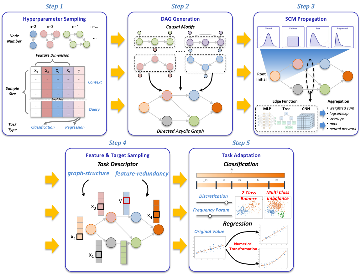
Because SCMs both define the DAG and the mechanisms, the pretraining distribution has an explicit causal structure that CCMM can, in principle, expose in the learned feature attention.
Results
Evaluation is on TabArena (51 datasets), TALENT (288 datasets after excluding 12 with >10 classes), and BCCO (156 datasets, with an emphasis on missingness and incomplete features), scored by Elo.
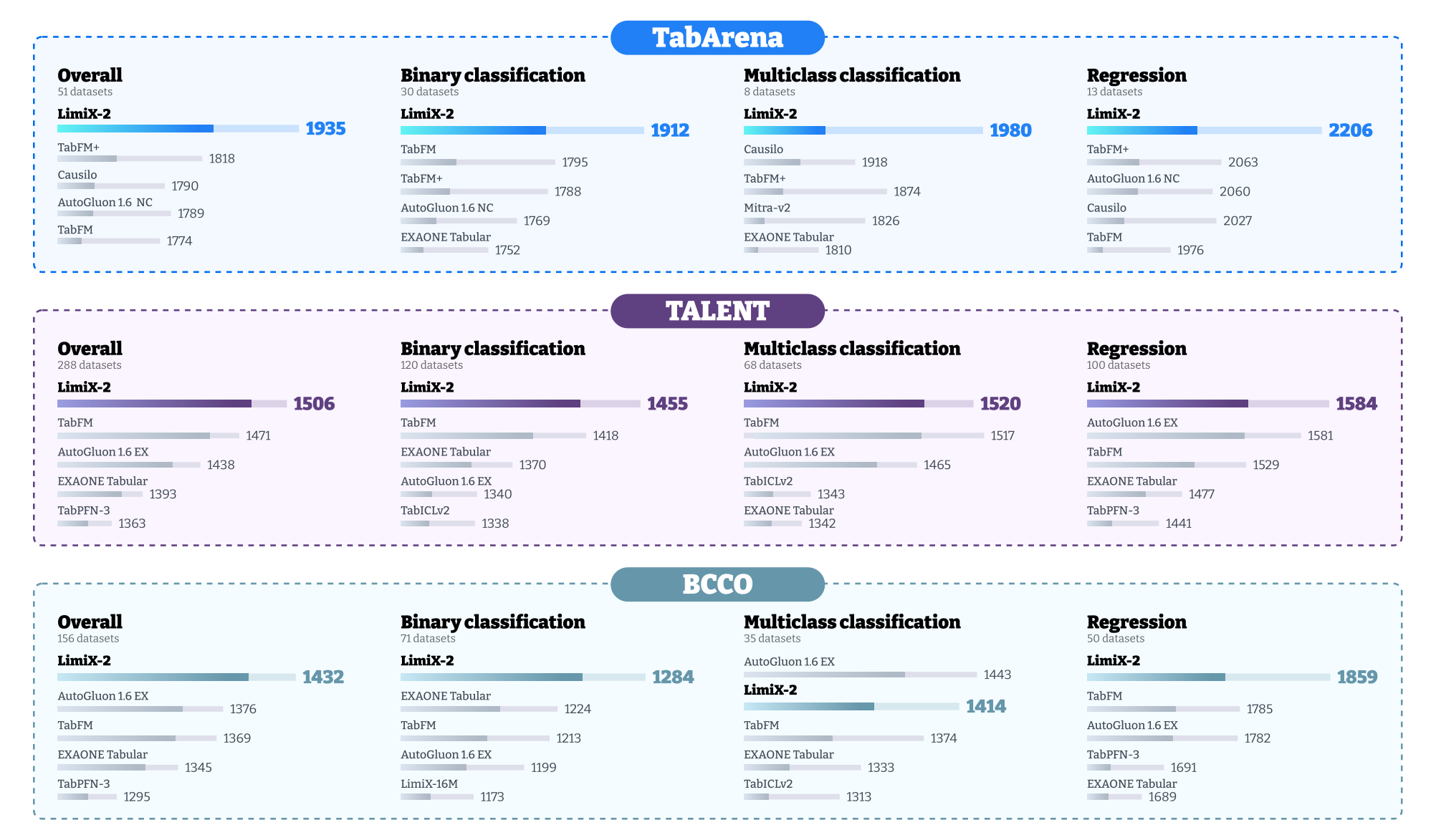
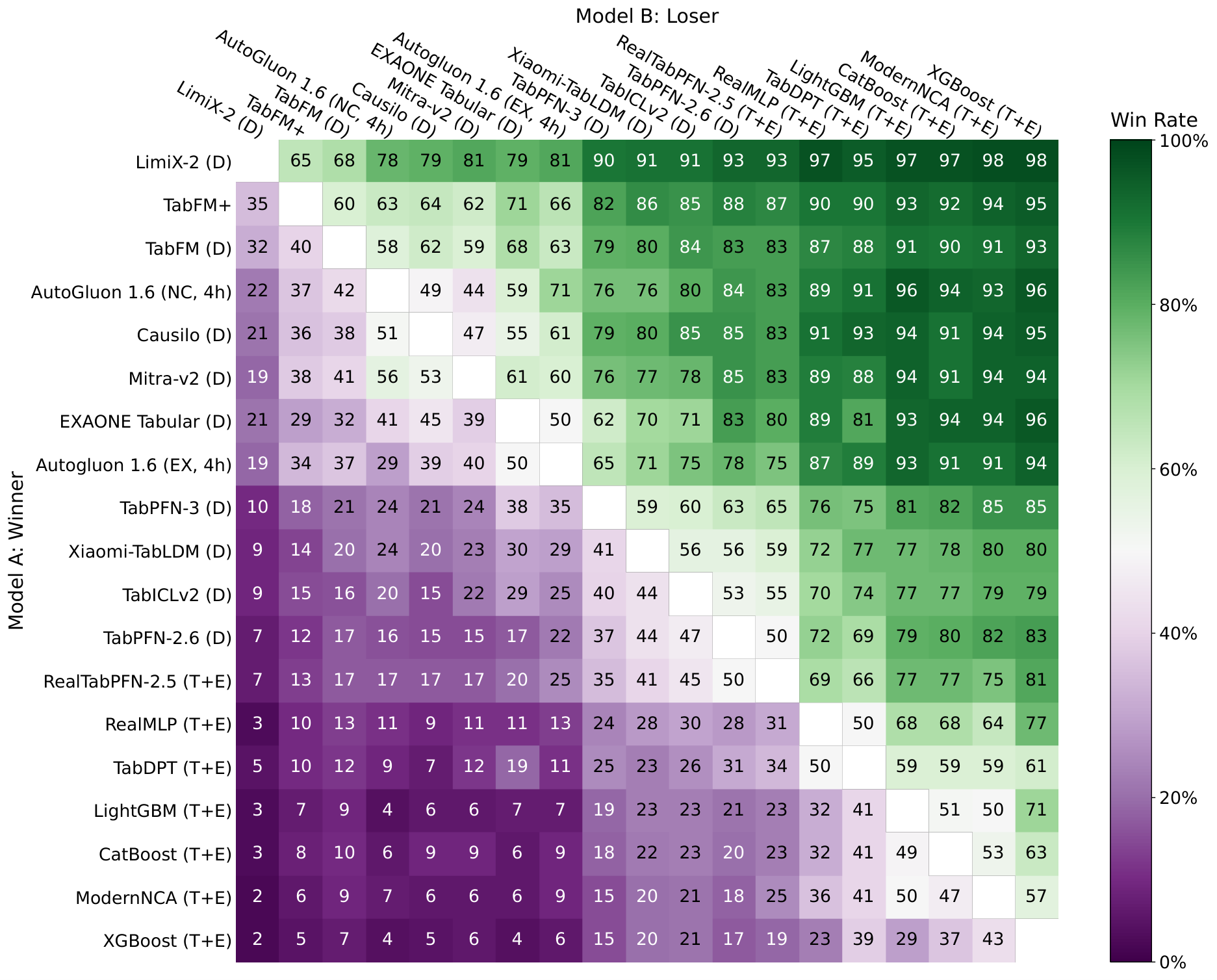
LimiX-2 attains Elo scores of 1935 on TabArena, 1506 on TALENT, and 1432 on BCCO, ranking first on all three, ahead of AutoGluon 1.6 and prior tabular foundation models. On TabArena’s pairwise view, every off-diagonal entry in the LimiX-2 row exceeds 60% win rate against each baseline.
Scaling. Fitting E_i=\alpha+\beta\log_2(N_i/100)+\varepsilon_i across six model sizes from 12.5M to 406.2M parameters gives clean log-linear fits: TabArena \alpha=1863.88,\ \beta=34.68,\ R^2=0.9808; TALENT-CLS \beta=22.16,\ R^2=0.9792; TALENT-REG \beta=18.26,\ R^2=0.9680; BCCO-CLS \beta=11.24,\ R^2=0.9617; BCCO-REG \beta=30.06,\ R^2=0.9702. Each doubling of parameters yields on the order of 10–35 Elo, with the largest returns on TabArena and BCCO-REG and the smallest on BCCO-CLS. The scaling data-generation and optimization recipe is held fixed, so these slopes are attributable to capacity alone.
Causal skeleton recovery. Using LimiX-2’s feature attention as an edge score, the recovered undirected causal skeletons outperform other tabular foundation models, XGBoost feature-importance baselines, and dedicated causal discovery methods on the evaluated benchmarks — a byproduct of learning p(\mathbf{x},y\mid D_{\mathrm{ct}}) under SCM-generated pretraining.
Limitations and open questions
The scaling coefficients differ substantially across benchmarks (BCCO-CLS \beta=11.24 vs. TabArena \beta=34.68), suggesting that missingness/robustness gains saturate faster than clean-task predictive gains. Extrapolation to the billion-parameter regime is fitted but not directly validated. The causal-skeleton claim rests on attention as a proxy for direct dependence; identifiability of edges under CCMM is not formally analyzed, nor is direction recovery. All pretraining is synthetic SCM data, so distributional coverage of real-world tabular idiosyncrasies (heavy-tailed categorical vocabularies, temporal leakage patterns) remains empirical rather than guaranteed. Finally, cell-level representations with N\times F\times d tensors scale poorly to very wide or very long tables; the paper widens the task FFN but does not report attention-cost mitigations at scale.
Why this matters
Reframing tabular in-context learning from p(y\mid \mathbf{x},D_{\mathrm{ct}}) to p(\mathbf{x},y\mid D_{\mathrm{ct}}) unifies prediction, imputation, anomaly scoring, and causal-skeleton discovery under one pretrained model, and the log-linear Elo scaling (R^2>0.96 across five task groups) suggests that structured-data foundation models admit predictable capacity scaling similar to LLMs — a useful planning signal for a subfield that has lacked one.
Source: https://arxiv.org/abs/2609.17488
Rethinking Critic Learning in PPO: Understanding and Mitigating Value Flattening
The failure mode
In PPO for LLM reasoning, the critic V_\phi(s) is trained on Monte Carlo returns from rolled-out trajectories and its predictions gate advantage estimates \hat{A}_t = R_t - V_\phi(s_t) (or the GAE variant). The authors document a systematic pathology: while MC-estimated state values \hat{V}^{\text{MC}}(s_t) swing sharply across adjacent reasoning steps — as should be expected when a chain of thought commits to or abandons a line of reasoning — the critic’s predictions across the same sequence are near-constant. They call this Value Flattening.
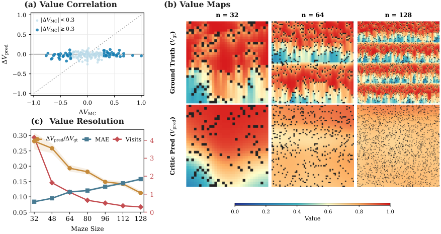
Figure 2(a) shows the mismatch directly on Qwen3-4B-Base trained on DAPO-Math-17k: on the x-axis, \Delta \hat{V}^{\text{MC}} between adjacent states spans the full [-1,1] range; on the y-axis, \Delta V_\phi collapses near zero. The critic misses both magnitude and sign of local value change. The consequence is that two reasoning states with very different true continuation values collapse to nearly the same baseline, corrupting the advantage signal that PPO’s policy gradient depends on.
Figure 2(b,c) confirms this is not an LLM-specific artifact. In a stochastic FrozenLake with maze size n \times n, the critic’s value map degrades as n grows even under a fixed training budget: ground-truth values retain sharp structure near the goal, critic maps smear out, and value-resolution statistics deteriorate monotonically with n. State-space size, not tokenization or reward sparsity, is the driver.
Mechanism
The paper attributes Value Flattening to two coupled effects in the standard dense critic loss
\mathcal{L}_V(\phi) = \frac{1}{T}\sum_{t=1}^{T}\big(V_\phi(s_t) - R\big)^2,
where all states s_1,\dots,s_T in a response share the same terminal return target R.
Implicit variance penalty. Because every state in the trajectory is regressed to the same scalar R, minimizing \sum_t (V_\phi(s_t) - R)^2 is equivalent (up to constants) to minimizing \sum_t (V_\phi(s_t) - \bar V)^2 + T(\bar V - R)^2 where \bar V is the empirical mean of critic outputs on the trajectory. The first term explicitly penalizes intra-response variance in critic predictions, biasing the critic toward flat profiles regardless of the true value trajectory.
Redundant updates from correlated states. Consecutive hidden states of an autoregressive LM are highly correlated, so their critic gradients \nabla_\phi V_\phi(s_t) point in nearly the same direction. Dense supervision then applies many near-parallel updates in a single step.
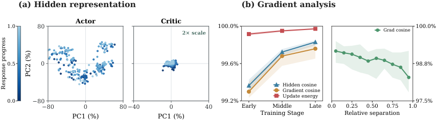
Figure 3 quantifies this: hidden-representation cosine alignment across adjacent states, gradient cosine alignment, and per-step update energy all remain high throughout PPO training. Redundant updates compound the variance-penalty bias — the critic learns a single trajectory-level scalar rather than a state-conditional function.
SP³O: sparse critic supervision
The fix follows directly from the diagnosis: supervise the critic on a small number of well-separated states per response. SP³O (SParse Proximal PPO) replaces the dense value loss with
\mathcal{L}_V^{\text{sparse}}(\phi) = \frac{1}{|\mathcal{S}|}\sum_{t \in \mathcal{S}}\big(V_\phi(s_t) - R\big)^2
with \mathcal{S} chosen at response-relative fractions \{0.3, 0.6, 0.9\}, adding a 0.95 anchor for responses of at least 6144 tokens to preserve late-tail coverage. This simultaneously (i) weakens the implicit intra-response variance penalty, since the mean-collapse term now involves only |\mathcal{S}|=3 or 4 terms, and (ii) removes most of the near-parallel gradient contributions.
The policy loss is unchanged; only critic supervision is sparsified. Advantages are still computed at every token using the (now better-resolved) critic.
Results
Experiments compare vanilla PPO, GRPO (critic-free), and SP³O on Qwen3-4B-Base and Qwen3-8B-Base trained on DAPO-Math-17k. With only three supervised states per response (plus the conditional 0.95 anchor), SP³O demonstrably reduces Value Flattening — the critic recovers non-trivial adjacent-state variation — and improves downstream policy performance consistently across both model sizes and multiple evaluation suites relative to standard PPO and GRPO. The paper reports gains across model sizes and evaluation suites; the mechanism is stable enough that the choice of three fixed relative positions works without per-task tuning.
Limitations and open questions
The paper fixes \mathcal{S} at hand-chosen relative positions rather than adapting to trajectory content — states where the reasoning actually branches are presumably more informative than the 0.3/0.6/0.9 quantiles. It is unclear whether the diagnosis extends to GAE with \lambda < 1, where bootstrapped targets differ across states and the shared-target argument weakens. The FrozenLake experiments show the effect grows with state-space size but do not establish scaling with model or context length in the LLM regime. Finally, the analysis treats the critic as a separate head; whether shared-backbone critics (common in practice) inherit the same pathology through gradient interference with the policy is not addressed.
Why this matters
Value Flattening reframes a widely-observed but poorly-understood PPO instability in LLM RL as a structural consequence of dense critic supervision on shared trajectory returns, and the fix — regressing on three states instead of thousands — is essentially free to deploy. It also partially explains why critic-free methods like GRPO have remained competitive: standard PPO critics have been actively miscalibrated.
Source: https://arxiv.org/abs/2609.18708
Flattening Every Memory Peak in Long-Context Mixture-of-Experts Training
Training MoE models at long context reveals a truth that average-footprint accounting hides: the run fails the moment any single tensor materialization exceeds HBM, and which tensor blows up first depends on the model, sequence length, and device count. This paper identifies four live sets that standard parallelism plans (ZeRO-3, sequence/context parallelism, expert parallelism, tensor parallelism) leave unbounded, and replaces each with a schedule whose GPU working set is fixed at launch. The design principle is uniform: each replacement operator must return bit-identical forward values and gradients, and its bound must survive checkpoint recomputation—so nothing sized by the routing matrix can be retained across the forward/backward boundary.
The four unbounded live sets
Section 2 tabulates them with per-rank sizes:
- Expert dispatch: 2 R_d H b bytes, where R_d is the number of routes received by destination d. Grows with batch, top-k, and router imbalance.
- Vocabulary projection: \mathcal{O}(NVb) logits from tokens \times vocabulary.
- Checkpoint boundaries: \sum_{\ell\in\mathcal{S}} N_\ell H b in HBM across depth \times length.
- Optimizer state: the 12\Theta/W bytes of Adam moments processed by a serial CPU update when offloaded.
None of these is bounded by sharding degree; each demands its own streaming schedule.
PipelinedLLEP: receiver-bounded dispatch
LLEP redistributes overflow from popular experts to idle ranks but still materializes the entire rank-local routed batch inside the all-to-all. PipelinedLLEP splits the batch into chunks under a per-source cap c:
K = \min(\lceil N/c\rceil, K_{\max}), \quad c_{\text{eff}} = \lceil N/K\rceil, \quad R_d^{(i)} \leq E_p k c_{\text{eff}}.
The bound depends only on E_p, k, and c_{\text{eff}}—router behavior cannot push any buffer past 2 E_p k c_{\text{eff}} H b bytes. Because K is derived from c, micro-batch length variation is absorbed in-flight without an OOM path. Chunking is contiguous rather than strided, exploiting LLEP’s property that a token’s destination is set by its position, so neighboring positions cluster to the same destination.
Ring-DTP for the vocabulary projection
For the logit head, the operator circulates activation or weight shards around a ring of P tensor-parallel workers, folding each strip of logits into an online log-sum-exp. In the move-weights variant (Figure 9), rank r keeps its batch (X_r, t_r) and running statistics S_r resident while each vocabulary block W_p hops around the ring; after P meetings every S_r is complete locally with no return hop. This drops the projection peak from \mathcal{O}(NVb) to \mathcal{O}(NVb/P) while preserving exactness of the loss and gradients.
Selective checkpoint offload and OffloadStreamAdamW
SCO keeps only the single long-lived tensor at each checkpoint boundary in CPU memory, capping HBM contribution from the checkpoint set at \leq 2 N_{\max} H b regardless of depth. OffloadStreamAdamW converts the serial CPU AdamW update into a bucketed pipeline of size \beta; the HBM footprint drops to \mathcal{O}(\beta) while host compute overlaps device compute rather than blocking it.
End-to-end composition
The four operators compose inside a MoP rank layout on 120B, 241B, and 667B MoE models across 16, 32, and 64 H200 GPUs. The baseline is FSDP2-best: the highest-throughput point of a full sweep over FSDP2 combined with expert, context, and tensor parallelism.
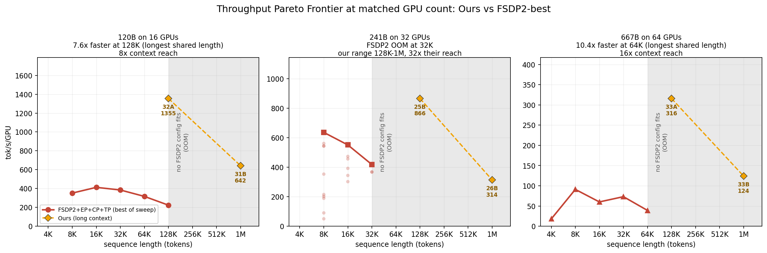
FSDP2-best exhausts memory past 128K, 32K, and 64K tokens on the three model scales; the composed stack trains at 1M tokens at all three, an 8\text{–}32\times context reach. At the longest length FSDP2-best still fits, the stack is 7.6\times faster at 128K on 120B and 10.4\times faster at 64K on 667B. The 241B case is starkest: FSDP2-best stops at 32K, four times shorter than the stack’s shortest configuration.
The FLOP-rate panel inverts the throughput trend because attention work per token scales with context. Per-GPU rate roughly doubles from 91\text{–}110 TFLOP/s at 128K to 213\text{–}233 TFLOP/s at 1M, while FSDP2-best never crosses 40 TFLOP/s anywhere in its sweep—about 2.2\times the baseline rate at 667B.
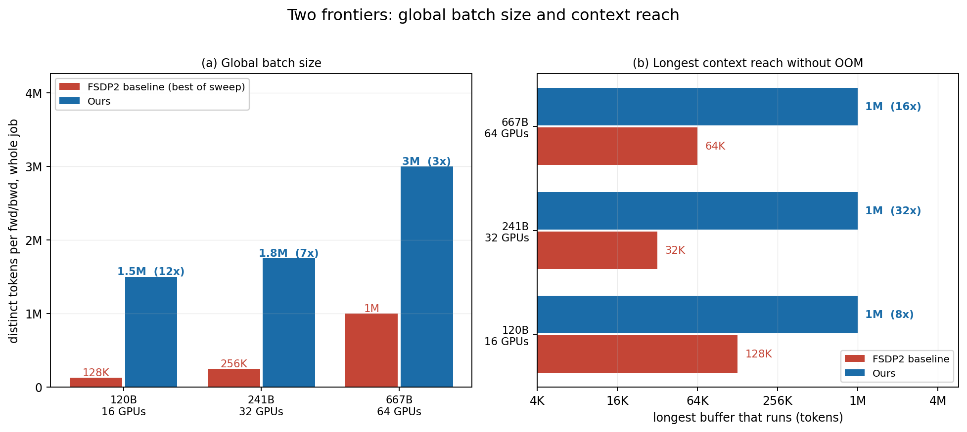
Figure 7 shows the frontier extension in both batch size and context, with the log-scale context axis making the multi-order gap visible.
Limitations and open questions
The evaluation is single-node scale (up to 64 H200), and Ring-DTP’s efficiency depends on ring bandwidth; behavior on multi-node fabrics with heterogeneous link speeds is unreported. SCO and OffloadStreamAdamW trade HBM for host-device PCIe bandwidth and CPU memory, and the paper does not characterize where the offload path itself becomes the bottleneck (e.g., very small \Theta/W or slow hosts). The 10% MFU dashed reference in Figure 6 highlights that even the composed stack sits below conventional dense-training utilization at short contexts; the win is reach, not peak arithmetic intensity. The operators require identical numerical outputs, but interactions with fp8/mixed precision accumulation for the online log-sum-exp deserve more discussion. Finally, PipelinedLLEP’s chunk-contiguity relies on LLEP’s position-to-destination mapping; the argument would need adjustment for routers whose destination is not a function of position.
Why this matters
Long-context MoE training is currently gated by whichever tensor happens to blow up first on a given configuration, and lowering one peak just exposes the next. This paper’s contribution is architectural discipline: bound every scaling axis with a launch-time-fixed working set, and the composition scales to 1M tokens on models where FSDP2 sweeps fall over at 32K.
Source: https://arxiv.org/abs/2609.14306
ScienceIDE: Turning World’s Scientific Codebase into Agent Learnable Environments
Scientific software—MHD codes, PIC solvers, DFT toolchains, stabilizer simulators—encodes methodological knowledge in executable form, but is largely inaccessible as agent training signal. Standard code benchmarks reward compilation and test-passing; scientific correctness requires physical invariants, numerical tolerances calibrated to the underlying discretization, and equivalence contracts that survive legitimate implementation variation. ScienceIDE is infrastructure that lifts pinned upstream repositories into environments where these criteria are enforced by executable checks, then uses the resulting verified trajectories for SFT and RL.
The construction pipeline
The unit of construction is a scientific module inside a versioned codebase: a coherent scientific responsibility (e.g., a Godunov flux stage, a particle push, a stabilizer decomposition) with executable coverage, owned implementation paths, and explicitly excluded responsibilities. An agent inspects a pinned revision, resolves dependencies, builds the source, runs official tests and examples to expose numerical variability and expensive paths, then proposes a module decomposition. A domain expert reviews boundaries and the equivalence contract; the registry enforces provenance but does not choose observables.
An approved module is packaged with (i) an editable agent workspace, (ii) public checks derived from official tests with calibrated pass policies, and (iii) a private verifier used at grading time. Task factories then specialize authoring procedures per environment, producing tasks that specify an initial workspace, a deliverable, and a verifier. The same check suite is reused across repair, implementation, acceleration, and reproduction task families—expert calibration is amortized.
Check calibration is the substantive design contribution. Pointwise comparison is used when measured sensitivity fits a scientifically meaningful window; invariants are used when pointwise bounds cannot contain valid variation without losing discrimination. Timings, adaptive step counts, rank layouts, and RNG draws are explicitly not observables. Nominal + variant initial conditions supply calibration evidence: each reference run must reproduce itself under an alternative legitimate build where available, and the observed spread informs (but does not automatically become) the tolerance. Each check carries a warrant stating what deviations it is intended to distinguish.
Inventory and evaluation
The frozen cohort spans 27 upstream codebases (Athena++, MITgcm, PLUTO, PHANTOM, LAPS, EPOCH, Meep, QuTiP, Stim, pymatgen, Gkeyll, EPREM, G4CMP, NEST, S4, pyAMG, PyXSIM, Basilisk, dscribe, EDKit.jl, eftcamb, Mink, Scirpy, SimuPy-Flight, strax, TSID, EDKit) yielding 64 environments and 2,812 tasks (2,515 repair, 295 implementation, 2 acceleration) with 1,076 executable checks.
ScienceIDE-Hard is a fixed 85-task cohort from 18 environments spanning five repository families: 33 MITgcm, 31 PLUTO, 11 LAPS, 9 Athena++, 1 PHANTOM. Success requires passing the private scientific checks, not just execution. Failure diagnostics reveal that termination status is uninformative: Qwen hits the budget on 37.3% of attempts and burns 48.5 min per unsuccessful episode; Haiku records no timeouts, averages 7.7 min per failure, and returns at or below the empty-delivery baseline on 74.9% of attempts; MiniMax combines low success with 31.6% timeouts and 34.1-min failures. Repeat instability is significant—28.0% of model–task pairs contain both success and failure within their first three valid attempts; Gemini flips outcome on 33/85 tasks vs. 8 for Astra and 29 for Kimi. Aggregate success rates thus conceal task-level unreliability.
Learning from scientific experience
The authors train PhAI-IDE-4B/9B/72B (from Qwen3.5-4B, Qwen3.5-9B, Qwen2.5-72B-Instruct) via SFT on GPT-5.6-sol trajectories filtered by numerical-equivalence verification. The corpus is task-identifier-disjoint: 4,567 training segments from 564 tasks, 544 validation segments from 81 tasks. Loss is applied only to new assistant tokens and tool calls in a target segment; instructions, observations, reused history, and trajectories flagged as failed/repetitive/extended-read-only are masked but retained as context. Training uses LoRA on all linear layers (r=32, \alpha=64, dropout 0.05), BF16, global batch 64, 36,864-token limit, lr 2\times10^{-5}, 3% warmup, cosine decay, three epochs (216 steps). Final checkpoints are used directly—no benchmark-based selection.
Validation loss drops from 0.383→0.340 (4B), 0.369→0.325 (9B), 0.401→0.313 (72B) between epochs 1 and 3, with final unmasked-target token accuracy of 91.12/91.33/92.01%.
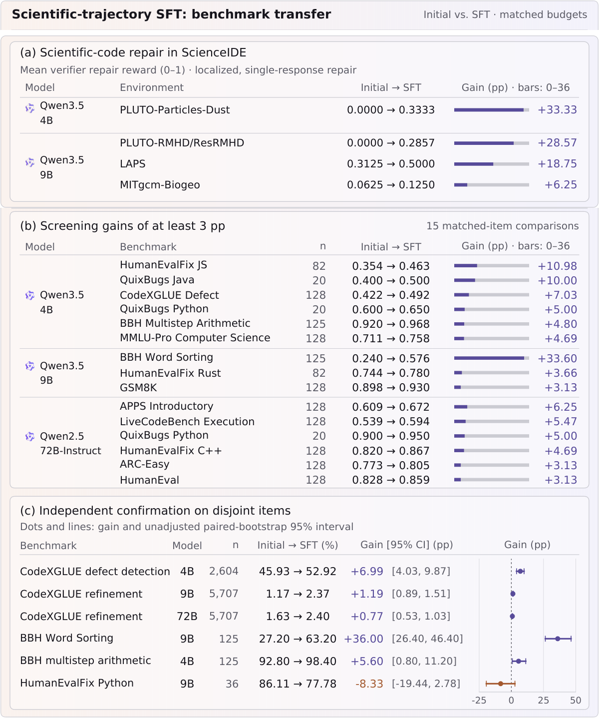
The more interesting result is transfer: SFT on verified scientific trajectories improves held-out ScienceIDE repair (mean verifier reward on 0–1 scale, reported as percentage-point gains) and produces ≥3 pp gains on 15 model–benchmark pairs across general code, reasoning, and knowledge benchmarks. This is evidence that experience grounded in physical/numerical verification transfers positively rather than overfitting to scientific idiosyncrasies.
Limitations and open questions
The acceleration family is essentially empty (2 tasks), so speedup-under-equivalence remains untested. ScienceIDE-Hard is dominated by two codebases (MITgcm + PLUTO = 64/85), and repository-family generalization is not disentangled from module-family generalization. Check calibration is expert-mediated and non-uniform across environments—warrants are auditable but not comparable across domains, complicating cross-environment reward aggregation. RL results are referenced but not shown in the excerpts, and the SFT teacher is GPT-5.6-sol, so distillation confounds are present. Repeat-instability numbers suggest evaluation stochasticity that any leaderboard built on ScienceIDE will need to control for explicitly.
Why this matters
Reliable agent learning in science needs verifiers that separate legitimate implementation variation from scientifically meaningful deviation; ScienceIDE operationalizes that with expert-calibrated executable checks reused across task families, and shows that training on the resulting trajectories transfers beyond the source domains. It is a plausible template for scaling verifiable RL/SFT signal from existing scientific codebases rather than synthetic tasks.
Source: https://arxiv.org/abs/2609.19134
ProgramDistill: From Interactive Web Apps to Verifiable Reference-Guided SWE Tasks
Existing coding-agent benchmarks (SWE-bench and descendants) assume the target behavior is specified textually — an issue, a docstring, a failing test. In practical web development, the specification is often another running system: a reference implementation whose source is opaque but whose behavior can be probed through a browser. ProgramDistill formalizes this setting as reference-guided software engineering: given a fully functional reference application and an editable current application with missing functionality, the agent must interact with the reference to infer intended behavior, then modify the current implementation to reproduce it.
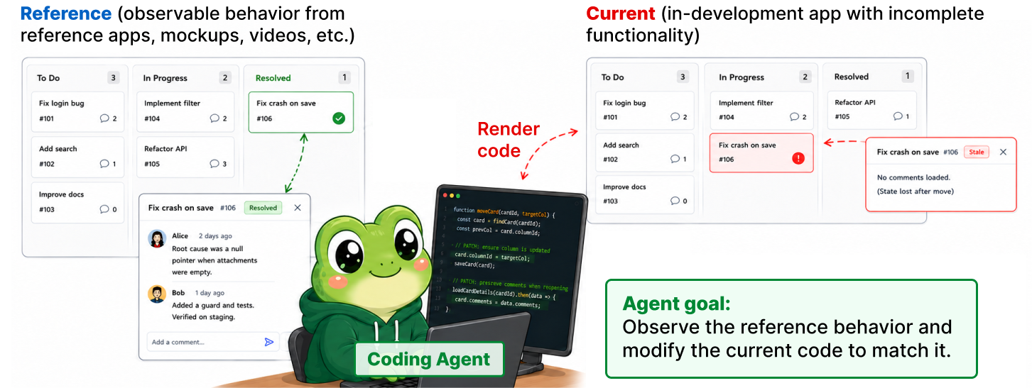
The core problem the authors solve is scalable construction of such tasks with automatic, ground-truth verification — no human-written issues, tests, or behavior annotations.
The mine–craft–patch pipeline
Each application is instantiated as a deterministic, browser-accessible execution environment providing (i) a stable reference for observation, (ii) an editable copy for task construction and repair, and (iii) a reproducible runtime for replay-based verification. All construction agents use GPT-5.6 Sol; the pipeline itself is model-agnostic.
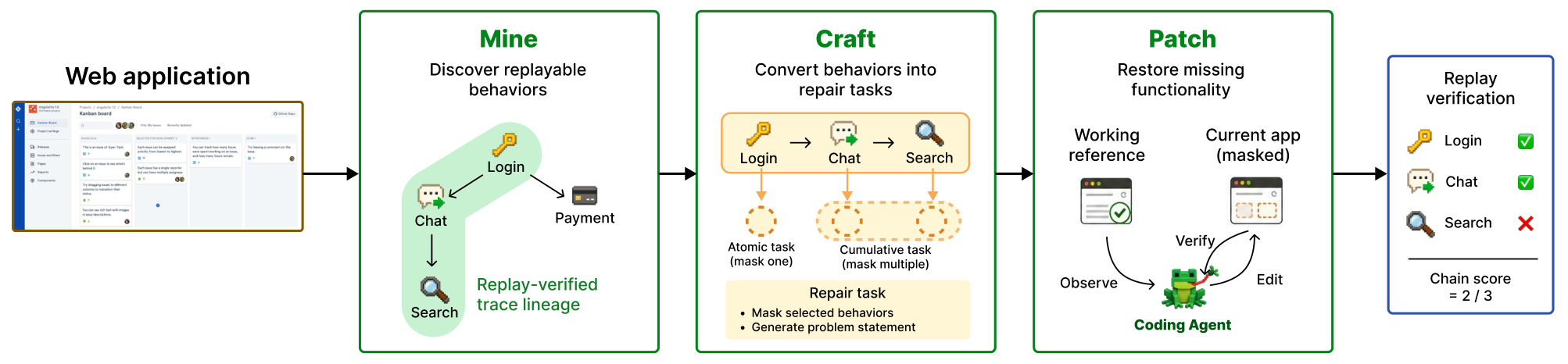
Mining proposes candidate behavioral goals and records interaction traces \tau that realize each goal. Because most nontrivial UI behaviors depend on prior application state (an account, a created board, etc.), mining does not treat traces as flat; it extends previously verified traces to produce new ones, forming a prerequisite trace tree. Each node’s execution requires replaying its ancestors as a bridge to establish state. Formally, a target trace at depth d requires a lineage (\tau_1, \tau_2, \ldots, \tau_d) where \tau_{i} is executable only after \tau_{<i} have been replayed. Figure 3 illustrates the concrete case in a Trello clone: account setup \tau_1 precedes board/card creation \tau_2, which precedes editor interaction \tau_3.

A candidate trace is admitted to the tree only if a clean-state replay reproduces it, and it must survive a second final replay check before being marked a verified behavior. This is the source of ground truth: each verified trace has a deterministic, replayable acceptance criterion.
Crafting produces tasks by masking. An atomic task masks exactly one behavior — the gold patch is the diff between the reference implementation of that behavior and its masked version. A cumulative task masks a lineage (\tau_1,\ldots,\tau_k) along the prerequisite tree, requiring the agent to restore an entire dependent chain. Masks are further partitioned by scope into logic-only and logic-and-UI, controlling whether the agent must reconstruct visual affordances as well as behavior.
Patching hands the coding agent the reference (behavior-observable) and the masked current application; after the agent submits edits, the pipeline replays the corresponding lineage traces and reports the fraction of the chain that succeeds. Because each trace has a deterministic replay verdict, evaluation is \{0,1\} per step, aggregated into per-lineage and cumulative success rates.
Benchmark statistics and results
Across 26 applications, mining proposes 2,800 candidate goals, collects 2,350 traces, of which 2,165 replay from a clean state, and 1,975 survive the final replay check. The resulting prerequisite trees reach a maximum lineage depth d=17 (mean 3.40), maximum width 60, and mean branching factor 1.78. Crafting emits 4,063 tasks split between atomic and cumulative variants, distributed over logic-only and logic-and-UI scopes.
On nine frontier coding agents, headline numbers:
- Full-application reconstruction, cumulative workflows. GPT-6 Astra reaches 49.2\% success; Claude Opus 5 reaches 28.8\%. The gap between top models on cumulative multi-step tasks is roughly 20 points, larger than typically seen on issue-style benchmarks.
- Partial-application reconstruction as a function of restoration depth. Success collapses with depth: from 100\% \to 64.0\% for the stronger model and 96\% \to 32\% for the weaker model as depth increases from 1 to 8. The near-perfect performance at d=1 indicates that atomic single-behavior repair from a live reference is largely solved for frontier models; the degradation with d isolates compositional reference-guided repair as the hard axis.
The depth-parameterized structure gives ProgramDistill a knob for controlled difficulty and makes it usable as a curriculum: cumulative lineages of increasing d provide a natural sequence of harder training targets, each with automatic verification.
Limitations and open questions
The pipeline’s coverage is bounded by what an LLM can propose as a goal and what the mining agent can drive the browser to execute; the drop from 2,800 candidates to 1,975 verified behaviors (\approx 29\% attrition) reflects both replay flakiness and coverage gaps. Verification is behavioral (replay of recorded traces), not semantic — an agent could pass by matching only the recorded interaction path rather than the general behavior. The corpus is 26 applications, heterogeneous but small relative to real-world web ecosystems. Finally, all construction relies on a single frontier LLM (GPT-5.6 Sol); systematic bias toward behaviors that model can articulate is likely and unquantified here.
Why this matters
ProgramDistill operationalizes a setting most SWE benchmarks ignore: specifications delivered as running software rather than text. The steep depth-vs-success curve exposes a compositional weakness in current agents that atomic-task benchmarks hide, and the fully automatic replay-verified pipeline makes it a plausible substrate for both evaluation and curriculum-style training on reference-guided repair.
Source: https://arxiv.org/abs/2609.18805
VC-Attention: Value Smoothing and Softmax Casting for Low-bit Attention
Attention dominates the deployment cost of video diffusion transformers because sequence length grows with spatiotemporal resolution. Existing low-bit attention kernels (SageAttention2/3, FlashAttention-4 in INT8/FP8) chase this cost, but two issues persist: (1) value tensors carry outliers with no exploitable channel or spatiotemporal structure, so per-block scales are wasted on a few large entries; (2) even when both matmuls are quantized to Tensor-Core precisions, the softmax between them — an FP32 exponential plus a downcast — becomes the longest pipeline stage. VC-Attention is a training-free framework that tackles both, keeping the online softmax recurrence intact.
The two residual bottlenecks
The motivation is quantified on Wan2.2: applying a Hadamard rotation to \mathbf{QK} shrinks the probability-side quantization error by 1.6×, but the \mathbf{PV} error is untouched and remains the larger of the two. Value quantization, not score quantization, bounds fidelity once QK is smoothed. Simultaneously, on B200 the FP32 exponentiation and cast between the two low-bit matmuls stays on the critical path, because Tensor Cores do not accelerate transcendentals.
V-Smooth: cluster, subtract, restore
Recall the FlashAttention online recurrence with block updates
m_i' = \max(m_i, \operatorname{rowmax}(\mathbf{S}_{ij})),\quad \alpha_i = \exp(m_i - m_i'), \widetilde{\mathbf{P}}_{ij} = \exp(\mathbf{S}_{ij} - m_i'),\quad \mathbf{A}_i \leftarrow \alpha_i \mathbf{A}_i + \widetilde{\mathbf{P}}_{ij}\mathbf{V}_j, l_i \leftarrow \alpha_i l_i + \widetilde{\mathbf{P}}_{ij}\mathbf{1},\quad \mathbf{O}_i = \mathbf{A}_i / l_i.
V-Smooth reorders value tokens by a lightweight online clustering so that each hardware block groups tokens with similar magnitudes. Within a block indexed by j, it subtracts the block-mean value vector \bar{\mathbf{v}}_j = \frac{1}{B}\sum_{t\in j}\mathbf{V}_t and quantizes only the residual \mathbf{V}_j - \mathbf{1}\bar{\mathbf{v}}_j^\top. The mean is folded back into the streaming numerator update through the row-sum the recurrence already maintains: since \widetilde{\mathbf{P}}_{ij}\mathbf{1}\bar{\mathbf{v}}_j^\top equals (block-mass) times \bar{\mathbf{v}}_j, one extra rank-1 accumulation restores it in FP32 without touching l_i. This turns per-block scale expenditure onto the tight residual distribution rather than absolute magnitudes, which is what makes value quantization work when outliers have no channel structure to smooth away.
ExpCast-FP8
The second contribution addresses the softmax stage. Rather than compute p = \exp(s - m') in FP32 and cast to E4M3 for the second matmul, ExpCast-FP8 emits the E4M3 code directly from the log-domain score. E4M3’s representable values are of the form 2^e (1 + m/8) for exponent e and 3-bit mantissa m. Since \exp(x) = 2^{x/\ln 2}, splitting x/\ln 2 into integer and fractional parts gives the E4M3 exponent and, via a small lookup on the fractional part, the mantissa. The FP32 exponential and the FP32→FP8 cast both leave the critical path.
Results
Fidelity is measured against BF16 FlashAttention-4 with matched seeds on Wan2.2-T2V-A14B (720p), LongCat-Video (480p), HunyuanVideo-1.5 (720p), and MiniMax-H3 (1344×768), 100 prompts each from MovieGen Bench.
On B200 8-bit, V-Smooth alone improves PSNR over SageAttention2 by +2.3 dB on Wan2.2 (22.6 vs 20.3), +1.4 dB on LongCat (24.5 vs 23.1), +2.8 dB on HunyuanVideo (18.4 vs 15.6), and +1.1 dB on MiniMax-H3 (21.0 vs 19.9). SSIM improves correspondingly (e.g. 0.792 vs 0.730 on Wan2.2) and LPIPS drops (0.152 vs 0.206). Adding ExpCast-FP8 costs some PSNR — Wan2.2 falls to 20.5, HunyuanVideo to 17.5 — but remains at or above the SageAttention2 baseline while removing the softmax bottleneck. The training-free Attn-QAT baseline at 4/8 precision is 3.4–6.7 dB below SageAttention2, confirming that naive lower-bit configurations without value-side treatment collapse.
On 4-bit workstation GPUs (RTX PRO 6000), V-Smooth gains are larger in relative terms: +2.9 dB on Wan2.2 over SageAttention3 (16.8 vs 13.9), +3.6 dB on LongCat (18.7 vs 15.1), +2.9 dB on HunyuanVideo (13.8 vs 10.9). Subject-consistency and imaging-quality metrics stay near BF16 across the board, as expected — they saturate on these models.

Kernel-level throughput on the same models translates the low-bit peak into wall-clock speedup on both datacenter and workstation cards, with the largest gains where SageAttention2 lacks a Blackwell kernel and falls back to older-GPU code (0.29× BF16 on B200 for MiniMax-H3).
Limitations and open questions
The online clustering adds preprocessing that the attention-only timings exclude but the clip wall-clock includes; the reported wall-clock margins therefore already price it in, but the paper does not decompose cluster cost by sequence length. ExpCast-FP8 trades ~1–2 dB PSNR for the removed FP32 stage, so the design point is workload-dependent — for MiniMax-H3 the drop is 0.8 dB, for HunyuanVideo 0.9 dB, both acceptable, but the crossover with training-based QAT at similar precision is not explored. The method is validated on video DiTs; language-model prefill/decode, where value distributions and softmax pressure differ, is out of scope. Finally, the interaction of V-Smooth’s block-mean recovery with numerical stability at 4-bit values is not analyzed in detail — the 4/4 PSNR numbers (13.8–18.7) suggest headroom remains.
Why this matters
Video DiT inference is bottlenecked by attention, and prior low-bit work optimized the \mathbf{QK} side while value outliers and FP32 softmax silently capped both accuracy and throughput. VC-Attention is a training-free, drop-in replacement that closes both gaps within the existing FlashAttention recurrence, which is the pragmatic path to deployable 8-bit and 4-bit video generation on current hardware.
Source: https://arxiv.org/abs/2609.15810
A Zeroth-Order Paradigm for LLM Preference Alignment
Problem: likelihood displacement in DPO-style objectives
Direct preference optimization and its variants collapse a preference pair (\mathbf{x}, \mathbf{y}^+, \mathbf{y}^-) into a differentiable loss on the log-likelihood margin \log \pi_\theta(\mathbf{y}^+|\mathbf{x}) - \log \pi_\theta(\mathbf{y}^-|\mathbf{x}). When the pair is noisy — meaning \mathbf{y}^+ and \mathbf{y}^- induce similar likelihoods under the current policy — the gradient of the DPO loss can drive both likelihoods down together (the “likelihood displacement” phenomenon), because the loss only constrains their difference. The authors’ remedy is to abandon the differentiable surrogate on such pairs entirely and instead extract a direction from the pair via a comparison oracle, plugged into a zeroth-order optimizer. The resulting method, ComPO, is meant to augment DPO/SimPO rather than replace them: clean pairs (large margin) still drive first-order updates; noisy pairs feed the oracle.
Method: comparison oracles and 1-bit sparse gradient estimation
For a comparison set S \subseteq D and two parameter vectors \theta, \theta', define the averaged preferred/dispreferred log-likelihood shifts
\Delta^{\pm}_S(\theta,\theta') = \tfrac{1}{|S|}\sum_{(\mathbf{x},\mathbf{y}^+,\mathbf{y}^-)\in S}\left(\log\pi_{\theta'}(\mathbf{y}^{\pm}|\mathbf{x}) - \log\pi_{\theta}(\mathbf{y}^{\pm}|\mathbf{x})\right).
The preference comparison oracle returns
\mathcal{C}^S_\pi(\theta,\theta') = \begin{cases} -1, & \Delta^+_S > 0 \text{ and } \Delta^-_S < 0, \\ +1, & \text{otherwise},\end{cases}
i.e., \theta' is preferred to \theta only when it strictly raises preferred likelihood and lowers dispreferred likelihood on average over S. Crucially, this is a \{\pm 1\} signal, not a scalar loss, and it is invariant to small equal shifts in both likelihoods — precisely the mode DPO fails on.
Given m random perturbations \{\mathbf{z}_i\}_{i=1}^m at radius r, ComPO queries y_i = \mathcal{C}^S_\pi(\theta_t, \theta_t + r\mathbf{z}_i) and forms the sparse 1-bit gradient estimate
\hat{\mathbf{g}} = \arg\max_{\|\mathbf{g}\|_1 \le \sqrt{s},\ \|\mathbf{g}\|\le 1} \sum_{i=1}^m y_i \mathbf{z}_i^\top \mathbf{g},
which enforces s-sparsity in \ell_1/\ell_2 sense on the estimated direction. The step \theta_{t+1} = \theta_t - \eta\hat{\mathbf{g}} is then applied. Theorem 3.2 gives a best-iterate convergence guarantee for the offline scheme under three assumptions: (i) there exists an \ell-smooth latent objective f that is compatible with the oracle in the sense that \mathcal{C}^S_\pi(\theta,\theta') = -1 whenever f(\theta') < f(\theta); (ii) \nabla f is approximately s-sparse, \|\nabla f(\theta)\|_1 \le \sqrt{s}\|\nabla f(\theta)\|; and (iii) an appropriate margin \Delta on oracle responses. The sparsity assumption is what makes the sample complexity in m tractable despite d being on the order of billions — updates concentrate on a low-dimensional subset of parameter coordinates.
Online ComPO retains this offline comparison direction on labeled pairs but interleaves a reverse-KL proxy computed on unlabeled generations from the current policy against a reference, giving a damping term analogous to the KL regularizer in RLHF. The performance guarantee for the constrained online scheme rests on local coverage (the reference distribution covers the optimizer’s neighborhood) and in-distribution pairwise reward accuracy.
Hyperparameters and empirical setup
The offline experiments split UltraFeedback pairs by margin threshold \delta_{\text{margin}}=3 into clean (DPO-updated) and noisy (ComPO-updated) subsets. Perturbation radii are small: r=5\times 10^{-4} for Mistral-7B and r=7.5\times 10^{-4} for Llama-3-8B / Gemma-2-9B, with m \in \{1600, 1800\} perturbations per update and sparse-regularization weight \lambda_g on the order of 10^{-4}. Training uses 30 A40 GPUs (46 GB each). Note m \approx 1600 oracle queries per step is substantial but each query is only a forward pass over S — no backward through the perturbed model is required, matching the zeroth-order premise.
Results
On AlpacaEval 2, Arena-Hard, and MT-Bench, augmenting a cleaned-DPO baseline with ComPO produces consistent gains. For Mistral-7B-Instruct, DPO_{\text{clean}}+ComPO reaches 26.17% LC / 18.32% WR on AlpacaEval 2, versus 23.89 / 16.15 for DPO_{\text{clean}} alone and 24.14 / 16.71 for vanilla DPO. The MT-Bench average jumps from 5.73 to 7.69 (Turn-1 6.11→7.78, Turn-2 5.34→7.63) — an unusually large gap that suggests either strong effects on follow-up coherence or judge variance worth scrutinizing.
For Llama-3-8B-Instruct, LC improves from 32.92 → 35.79% and Arena-Hard WR from 22.9 → 23.1, with MT-Bench average 7.94 → 8.05. On Mistral-7B-Base and Llama-3-8B-Base the picture is similar but smaller in magnitude: e.g., Mistral-7B-Base AlpacaEval 2 LC 9.41 → 11.66 with ComPO. Arena-Hard on Llama-3-8B-Base is flat (12.0 → 12.1).
Limitations and open questions
Several issues merit caution. First, the convergence guarantee relies on the existence of an \ell-smooth latent f compatible with the oracle everywhere, plus approximate gradient sparsity — neither is verified empirically for LLM parameter spaces, and the sparsity assumption is what actually makes m=1600 enough. Second, the Mistral-7B-Instruct MT-Bench delta (5.73 → 7.69) is large relative to the AlpacaEval / Arena-Hard deltas on the same model, raising questions about MT-Bench judge stability across single runs; the paper notes ablation tables report run-to-run variation, but the main table reports point estimates. Third, ComPO’s compute cost per step scales linearly in m; the practical cost/quality trade-off versus simply cleaning noisy pairs and discarding them is not directly benchmarked. Finally, oracle-compatibility is defined pointwise but only verified through downstream metrics — pairs where \Delta^+ > 0, \Delta^- < 0 can still be locally misleading.
Why this matters
Likelihood displacement is a real failure mode of margin-based preference losses, and ComPO offers a principled alternative that preserves the sign information in noisy pairs without inventing a scalar loss on them. The zeroth-order/comparison-oracle framing also opens a route to alignment with non-differentiable or human-in-the-loop feedback, where only ordinal comparisons are available.
Source: https://arxiv.org/abs/2609.19144
Hacker News Signals
Breaking the 1.58-bit Barrier for Ternary LLMs
Source: https://arxiv.org/abs/2609.16338
The standard BitNet b1.58 formulation constrains weights to \{-1, 0, +1\}, achieving \log_2 3 \approx 1.58 bits per parameter. This paper asks whether that entropy ceiling is actually load-bearing or just a convenient quantization grid.
The core contribution is a revised training and packing scheme that treats ternary weights not as a fixed alphabet but as a distribution over that alphabet that can be entropy-coded. Given a learned weight distribution p(-1), p(0), p(+1) with entropy H < 1.58 bits, arithmetic coding can pack the weight tensor below the naive 1.58-bit floor. The authors show that typical trained ternary networks skew heavily toward zero — sparsity in the ternary sense — so the actual entropy is often in the 1.1–1.4 bit range, and that gap is recoverable.
The method combines: (1) straight-through estimator training with an explicit entropy regularization term added to the loss, pushing the weight distribution toward lower entropy without collapsing to binary; (2) a block arithmetic coder at inference time that amortizes overhead across 256-weight blocks; and (3) a lookup-table GEMM kernel that operates directly on the packed representation, deferring decode to accumulation time.
On LLaMA-architecture models at 1B–7B scale, they report perplexity matching or within 0.3 points of full 1.58-bit baselines at 1.2–1.35 effective bits per weight. Memory reduction over the 1.58-bit baseline reaches 15–25% depending on the zero-fraction achieved. Throughput on CPU inference improves by roughly 10–18% due to reduced memory bandwidth pressure.
The limitation is that the arithmetic coding/decoding adds latency that only pays off when memory bandwidth is the bottleneck — on high-bandwidth accelerators the gains shrink or invert. The entropy regularization hyperparameter also requires tuning per model scale.
Why this matters
Compressing below the ternary entropy ceiling without accuracy loss reframes 1.58-bit as a soft target rather than a hard constraint, opening a continuous tradeoff curve between weight entropy and model quality.
Training a 4B Model to Produce 81% Faster Query Plans than Postgres
Source: https://rohanbansal.com/qorl
This project applies reinforcement learning to learned query optimization, targeting the specific failure mode where Postgres’s cost-based planner produces suboptimal join orders and index selection under skewed or correlated data distributions.
The setup: a 4B-parameter transformer is trained with RL to output query execution plans (represented as serialized operator trees) for a fixed schema. The reward signal is negative wall-clock execution time measured against an actual Postgres instance. The model takes as input the SQL query plus schema statistics (table cardinalities, column histograms, foreign key graph) and autoregressively generates a plan in a DSL that maps to Postgres’s pg_hint_plan extension, forcing the executor to follow the model’s choices.
Training uses a variant of GRPO (group relative policy optimization) rather than PPO, avoiding a separate value network. A group of K=8 plan candidates is sampled per query, ranked by execution time, and the policy gradient is computed against group-normalized rewards. The training corpus is generated synthetically: random SQL queries over the TPC-DS and Stack Overflow schemas with injected data skew.
The 81% speedup figure is a geometric mean over a held-out query workload where Postgres is given default statistics (no ANALYZE tuning). On well-analyzed schemas the gap closes to roughly 23%. The model underperforms on queries involving more than 12-way joins — plan space explosion causes the autoregressive decoder to produce invalid operator trees at non-trivial rates, requiring a constrained decoding layer.
Latency of the model itself (plan generation time) adds ~40ms per query, which is only acceptable for OLAP workloads. The approach does not generalize across schemas without fine-tuning.
Why this matters
Demonstrates that RL-from-execution-feedback can beat a mature cost-based optimizer on realistic workloads, but surfaces the schema-specificity problem as the central unsolved obstacle to deployment.
Nvidia Announces Native GPU Programming in Rust
Source: https://developer.nvidia.com/blog/introducing-cuda-rust-two-tracks-for-writing-gpu-kernels/
Nvidia is shipping two distinct integration paths, and conflating them misrepresents what is actually available.
Track 1 is cuda-std, a Rust crate that provides safe wrappers around CUDA intrinsics and exposes them through standard Rust abstractions. Kernels are written in ordinary Rust, compiled to PTX via rustc’s NVPTX backend (which has existed since 2017 but was never officially supported). The new piece is Nvidia taking ownership of the toolchain integration: a nvcc-compatible driver wrapper that handles device/host code splitting, and a set of #[kernel] proc-macro attributes that generate the required ABI boilerplate. Memory safety guarantees apply only to host-side code; device-side Rust is unsafe by default because CUDA’s execution model (warp divergence, shared memory aliasing, syncthreads barriers) does not fit Rust’s ownership model.
Track 2 is a lower-level PTX emission path where Rust code is compiled to an IR that Nvidia’s own compiler then optimizes, closer to how MLIR-based stacks like Triton work. This is aimed at library authors who need deterministic register allocation and want to avoid rustc’s LLVM backend making unexpected spilling decisions.
Neither track supports the full CUDA C++ ecosystem (cooperative groups, tensor core intrinsics via nvcuda::wmma) at launch. The tensor core path is listed as “planned.” Existing cuBLAS/cuDNN calls from Rust go through FFI as before.
The practical significance is toolchain legitimacy rather than new capability: the NVPTX backend already worked, but without Nvidia’s blessing and without integration into nvcc’s multi-file compilation model, shipping production kernels in Rust was fragile.
Why this matters
Official vendor support removes the primary adoption barrier for Rust in GPU compute; whether Rust’s ownership model can be made ergonomic for SIMT programming remains an open design problem.
Dream-RSI: Recursive Self-Improvement Through Evolving Worlds
Source: https://arxiv.org/abs/2609.14858
The paper formalizes recursive self-improvement (RSI) as a curriculum problem: an agent that improves its own training environment to maximize long-horizon capability gain, rather than having a human engineer the curriculum externally.
The architecture is a dual-loop system. The inner loop is a standard RL agent (transformer policy) learning a task within a parametric world model. The outer loop is a second model — also a transformer — that modifies the world model parameters to maximize a meta-objective. The meta-objective used is not final task reward but learning progress: the derivative of inner-loop performance with respect to training steps, approximated as (R_{t+k} - R_t)/k over a window.
The world model is a discrete-state simulator (a 2D grid world with configurable object interactions) whose parameters control difficulty, reward density, and transition stochasticity. The outer-loop model is trained with evolutionary strategies (CMA-ES), not gradient descent, because the mapping from world parameters to inner-loop learning curves is non-differentiable.
Results are reported on a suite of navigation and tool-use tasks. The RSI loop discovers curricula that produce agents reaching human-level performance on held-out task variants roughly 3x faster (in inner-loop steps) than fixed curricula or domain-randomization baselines. The outer-loop model itself is retrained every N=500 inner episodes, creating the “recursive” element.
Limitations are significant: the world model is hand-coded and narrow, the outer loop has not been tested on continuous-action domains, and there is no mechanism preventing the outer loop from collapsing to trivially easy worlds that maximize short-horizon learning signal.
Why this matters
Provides a concrete, reproducible instantiation of the RSI loop with measurable curriculum quality metrics, though the gap to general self-improvement is large.
Intelligence per Watt: Measuring Intelligence Efficiency of Local AI
Source: https://arxiv.org/abs/2511.07885
The paper proposes a measurement framework for intelligence efficiency — benchmark performance normalized by energy consumption — for locally-run LLMs, targeting hardware comparison rather than model comparison.
The core metric is \eta = S / P_{\text{avg}}, where S is a composite benchmark score (average of MMLU, HellaSwag, ARC, and GSM8K normalized to [0,1]) and P_{\text{avg}} is average power draw in watts measured at the wall socket during inference. Tokens-per-second is tracked separately but not folded into \eta to avoid conflating throughput with quality.
The authors run a standardized harness across a matrix of hardware (Apple M-series, AMD Ryzen AI, Intel Core Ultra, Nvidia RTX consumer GPUs) and quantization levels (fp16, int8, int4, GGUF Q4_K_M, Q8_0) using llama.cpp and ollama as runtimes. Power measurement uses a MQTT-connected smart plug logging at 1Hz, which introduces measurement noise at the ~1W level — acceptable for the 15–120W range of devices tested.
Key findings: Apple M4 Pro achieves the highest \eta across all tested configurations, roughly 2–3x better than discrete GPU configurations at comparable benchmark scores, primarily due to unified memory eliminating PCIe transfer overhead and Apple’s low idle power floor. Int4 quantization improves \eta over fp16 by 40–60% on GPU with less than 2 percentage point benchmark degradation. The framework explicitly excludes embodied carbon and amortized hardware cost.
The 1Hz power logging granularity is a real limitation for bursty prefill/decode workloads. The composite benchmark score is also a crude proxy for “intelligence.”
Why this matters
Establishes a reproducible methodology for hardware purchasing decisions based on energy efficiency rather than raw throughput, relevant as local inference becomes a cost-sensitive deployment target.
Vectorized and Performance-Portable Quicksort (2022)
Source: https://opensource.googleblog.com/2022/06/Vectorized%20and%20performance%20portable%20Quicksort.html
Google’s Highway-based Vqsort is a SIMD quicksort that achieves performance portability across AVX-512, AVX2, NEON, and SVE without separate codepaths, using the Highway abstraction layer.
The algorithm combines two SIMD-friendly primitives. First, a sorting network for small fixed-size blocks (16–256 elements depending on register width) implemented with Highway’s SortByKey and conditional swap operations that compile to VPERMD/VPBLENDVPS on AVX-512 and equivalent instructions on other targets. Second, a vectorized partition step that replaces the scalar pivot-comparison loop: given a pivot p, all elements in a vector register are compared simultaneously, and a compress-store (CompressStore in Highway) writes the less-than and greater-than partitions to separate buffers in a single pass with no branch per element.
The partition throughput is the bottleneck on large arrays, and the compress-store eliminates the scalar scattering that makes branch-based partitioning pipeline-unfriendly. AVX-512’s VPCOMPRESSD makes this direct; on AVX2 it is emulated with a lookup-table-based shuffle, incurring roughly 2x overhead but still outperforming scalar.
Benchmarked on 10M float32 elements, Vqsort is 5–10x faster than std::sort (introsort) on AVX-512 hardware and 1.5–3x faster on AVX2. The portable implementation means a single binary runs efficiently on all targets via runtime dispatch.
The resurfacing on HN prompted discussion of the 2025 follow-on work extending Vqsort to key-value pairs and 128-bit types, and comparisons with NVIDIA’s CUB radix sort (which wins on GPU but requires data on device).
Why this matters
Demonstrates that performance-portable SIMD code via Highway can match hand-tuned platform-specific implementations, validating the abstraction layer approach for compute-intensive primitives.
Recreating Voodoo Graphics and a Late-1990s Gaming PC on an FPGA
Source: https://nand2mario.github.io/posts/2026/zsst-voodoo/
This is a full-system FPGA implementation targeting accurate reproduction of a 1998-era gaming PC with a 3dfx Voodoo Graphics (VSA-100 architecture) add-in card.
The implementation runs on a Xilinx Artix-7 board and consists of several independent RTL modules wired together: an x86 core (using an existing open-source 486-compatible softcore), ISA/PCI bus fabric, VGA controller, and the Voodoo Graphics subsystem. The Voodoo Graphics module is the novel contribution and is the most technically involved piece.
The Voodoo Graphics architecture has two processing units: the FBI (Frame Buffer Interface) and the TMU (Texture Mapping Unit). The FBI handles triangle setup and rasterization; the TMU handles perspective-correct texture sampling with bilinear filtering. Implementing perspective-correct texturing in RTL requires a per-pixel divide (u/w, v/w) — the author uses a pipelined Newton-Raphson reciprocal unit to avoid a full divider, matching the original chip’s approach. The texture cache is a direct-mapped 8KB SRAM block, and cache miss handling is the dominant source of cycle-count divergence from original hardware.
The Glide API (3dfx’s proprietary graphics API, which games called directly rather than going through DirectX) is emulated at the PCI command-register level: a software shim running in the x86 softcore intercepts Glide calls and translates them to register writes to the FPGA’s Voodoo module.
Gate utilization on the Artix-7 is approximately 78%, leaving little headroom. Several games run with visual accuracy within 1–2% of reference captures; alpha blending and fog effects show the largest divergence due to timing differences in the TMU pipeline.
Why this matters
Demonstrates that a complete heterogeneous system from this era is now tractable on a mid-range FPGA, and the RTL serves as a clean reference implementation for Voodoo’s rendering pipeline that no longer requires physical hardware.
Noteworthy New Repositories
tigerless-labs/agent-memory
A long-term memory runtime for AI agents that uses plain Markdown files as the canonical store rather than a vector database or proprietary API. Retrieval is local and ranked — the library scores chunks by recency, relevance, and explicit importance tags without requiring an embedding service. The architectural highlight is a separate “sleep-time” Manage layer that runs asynchronously to consolidate, deduplicate, and re-rank stored memories, mimicking offline memory consolidation rather than doing it inline during inference. Both Claude Code and OpenAI Codex can share the same store simultaneously via a common interface, which matters for multi-agent pipelines where context continuity across sessions is otherwise lost. Because everything is Markdown, the memory store is human-readable and version-controllable with standard tooling. No external API key is needed, making it viable for air-gapped or cost-sensitive deployments. The design prioritizes debuggability: you can inspect exactly what an agent “remembers” by reading files. The ranked retrieval appears to use a BM25-style lexical approach combined with recency decay, avoiding the operational overhead of embedding pipelines. Primary use case is persistent agent workflows where task state, user preferences, and intermediate results need to survive across sessions.
Source: https://github.com/tigerless-labs/agent-memory
shinthink/blitzstrike
A Model Context Protocol (MCP) server exposing a structured penetration-testing methodology to any MCP-compatible AI agent. The catalog contains 130 tools organized into phases: reconnaissance and attack-surface mapping, source-to-sink taint analysis for code-level vulnerabilities, and live validation of findings. The “57 escalation chains” are pre-encoded sequences of tool calls that chain lower-severity findings into privilege escalation paths, reducing the manual reasoning burden on the agent. The intelligence data layer appears to store reusable artifacts — discovered endpoints, credentials, service fingerprints — across tool invocations so later steps can reference earlier findings without re-running scans. Because it exposes a single MCP server, any agent framework (Claude, GPT-4o function calling, open-source LLM with tool use) can consume it without per-agent integration work. The structured methodology encoding is the substantive contribution: rather than a flat list of tools, it encodes domain knowledge about attack sequencing. Useful for red-team automation research, security labs, and CTF pipelines where repeatability and agent-driven enumeration are the goals.
Source: https://github.com/shinthink/blitzstrike
S1N6H/pentest-harness
A self-hosted orchestration harness that wraps an arbitrary AI model (via bring-your-own API key) into a session-persistent penetration testing agent. The design keeps all session data local — scan results, tool outputs, conversation history — which matters for authorized engagements where data exfiltration to third-party services is prohibited by scope agreements. The harness targets bug bounty hunting, CTFs, and internal security labs rather than production red-teaming at scale. Architecturally it acts as a thin controller: it manages tool dispatch (likely wrapping standard tools like nmap, ffuf, nuclei), feeds outputs back to the model with structured prompts, and persists session state between invocations so an operator can resume mid-engagement. The “bring your own model” approach means it works with any OpenAI-compatible endpoint, including locally hosted models via Ollama or LM Studio, which is relevant for classified or sensitive environments. Compared to blitzstrike above, this is a harness rather than a tool catalog — it provides the agent loop and session management rather than encoding attack methodology. Practical for security researchers who want agent-assisted enumeration without cloud dependency.
Source: https://github.com/S1N6H/pentest-harness
useagenthq/useagent
An open-source agent runtime that provisions each agent with an isolated cloud computer — a sandboxed environment with a browser, filesystem, and shell — so agents can execute multi-step tasks that produce real artifacts: websites, spreadsheets, slide decks, pull requests. The runtime dispatches to Claude Code, OpenAI Codex, or OpenCode using the operator’s own subscription credentials, avoiding vendor lock-in at the model layer. The “AI coworker” framing reflects the technical design: agents receive team context (tools, codebases, data sources) and return finished work rather than intermediate steps, with the cloud computer handling execution isolation. This is meaningful for tasks that require stateful browser interaction or file I/O that pure API calls cannot handle. The open-source nature means the sandboxing and tool integration layer is auditable, which matters for teams handling sensitive codebases. Architecturally similar to Anthropic’s computer use demos or OpenDevin, but positioned as a team-deployable runtime rather than a research prototype. Key differentiator over hosted alternatives is that compute and model costs stay on the operator’s existing accounts.
Source: https://github.com/useagenthq/useagent
jtydhr88/screenwriting-skills
A collection of agent skill definitions targeting professional screenwriting, television writing, and dramaturgy workflows. The substantive content is structured prompt templates and tool-use schemas encoding domain knowledge: three-act and five-act structure analysis, scene breakdown, character arc tracking, dialogue revision, and format-compliant script output (Final Draft / Fountain conventions). At 1,216 stars it has found a clear niche among writers using LLM-assisted drafting. The skills are likely designed for integration with agent frameworks that support modular skill loading — each skill is a discrete, composable unit rather than a monolithic prompt. The dramaturgy angle is notable: it goes beyond pure script formatting into structural analysis tasks (identifying dramatic beats, tracking thematic consistency) that require multi-pass reasoning over long documents. For researchers interested in creative long-form generation, this repository provides a curated set of domain-specific evaluation criteria and task decompositions. Practically useful for anyone building a writing assistant where generic instruction-following models lack structured knowledge of professional script conventions.
Source: https://github.com/jtydhr88/screenwriting-skills
OnlyTerp/opengrok
A client-side wrapper that enables running arbitrary models through Grok Bot’s interface, including a model-picker UI and provider wire maps that route requests to the appropriate backend. The “update-proof doctor” component is a self-diagnostic that checks whether the underlying provider mappings are still valid after Grok Bot updates, reducing maintenance burden as the upstream API evolves. The “evidence-based provider wire maps” suggests the routing logic is documented and verifiable rather than reverse-engineered heuristics, which makes it more maintainable. The one-command setup lowers the friction for users who want model flexibility without building their own API integration layer. The project’s value is primarily in the aggregated reverse-engineering work and the maintained compatibility layer — the technical substance is in the wire maps and the doctor tooling rather than novel algorithms. Useful for developers who want to prototype against multiple providers through a single interface, or for users who want access to models not natively exposed through Grok’s standard UI.
Source: https://github.com/OnlyTerp/opengrok
pax-beehive/dsh-hub-cli
A CLI, schema definitions, resolver, and agent tooling for a DSH (Data Science Hub or Domain-Specific Hub) Plugin Hub ecosystem. The core components — CLI for plugin management, schemas for plugin contracts, and a resolver for dependency and version resolution — follow the standard plugin registry pattern seen in package managers and VS Code extension systems. The agent tools layer suggests plugins can be invoked by AI agents programmatically, making this a tool registry rather than purely a developer distribution channel. The open-source nature of the resolver and schemas means plugin authors can validate compatibility locally and understand exactly how resolution decisions are made. The CLI likely handles authentication, publish, install, and update operations against the hub. For teams building modular agentic systems where capabilities are packaged as plugins, a well-specified schema and resolver prevents the dependency hell that plagues informal tool catalogs. The project appears to be infrastructure for a broader DSH ecosystem; its value depends on what plugins are available and whether the hub backend is also accessible.
Source: https://github.com/pax-beehive/dsh-hub-cli
monid-ai/monid
Positions itself as an OpenRouter-equivalent for agent tools rather than models: a unified routing and abstraction layer that normalizes access to heterogeneous tool APIs behind a single interface. Where OpenRouter aggregates LLM providers, Monid aggregates tool providers — external services, data sources, action endpoints — so an agent developer writes against one schema rather than per-provider integrations. The technical substance lies in the normalization layer: schema translation, authentication management across providers, and routing logic that selects the appropriate backend based on capability requirements or cost. This matters because tool fragmentation is a genuine pain point in multi-agent systems — agents built against one tool provider’s schema break when that provider changes or when a team wants to swap backends. A routing layer with a stable interface decouples agent logic from tool implementation details. At 224 stars it is early, and the utility depends heavily on the breadth of tool providers supported and the fidelity of the schema normalization. For teams running heterogeneous tool stacks, the concept addresses a real integration tax.