Daily AI Digest — 2026-09-16
arXiv Highlights
Continual Learning Mechanisms Compose for Long-Horizon Memorization
Problem
The paper studies a stringent continual learning regime: 100 sequential supervised fine-tuning tasks, each a set of query-answer pairs to be memorized, with no replay buffer of raw examples and no task ID at inference (domain-incremental). Evaluation is on the training set of each task — this is a memorization benchmark, not a generalization one. The motivation is practical: models increasingly need to internalize streams of factual updates (test-time training, agent memory, incremental knowledge editing) and to retain them across many subsequent updates. At T=100, standard continual learning mechanisms individually collapse to near-zero retention.
The core hypothesis is that catastrophic forgetting has multiple, complementary sources, and mechanisms that address different sources should compose additively. The authors organize the design space along two axes: anchors (what prior information each update preserves) and low-rank allocation rules (where successive updates are stored in the parameter space).
Method
Each task t arrives with data \mathcal{D}_t and the model minimizes
\Theta_t = \arg\min_{\Theta}\ \mathcal{L}_{\mathrm{SFT}}^t(\Theta) + \mathcal{R}_D^t(\Theta) + \mathcal{R}_F^t(\Theta) + \mathcal{R}_W^t(\Theta),
with \mathcal{L}_{\mathrm{SFT}}^t = -\mathbb{E}_{(x,y)\sim\mathcal{D}_t}[\log p_\Theta(x,y)] (unmasked over the query, since query/answer segmentation is not always available). The three regularizers correspond to:
- Data anchor \mathcal{R}_D: generative replay from earlier task heads/prompts, no stored raw examples.
- Function anchor \mathcal{R}_F: distillation-style penalty matching prior predictive distribution on anchor inputs.
- Weight anchor \mathcal{R}_W: parameter-space penalty (SI-style importance-weighted quadratic to \Theta_{t-1}).
The second axis is low-rank allocation over LoRA adapters:
- Shared LoRA: single adapter reused for every task (most interference).
- Merged LoRA: after each task, merge the current LoRA delta into the base weights; allocate a fresh LoRA for the next task. Retained state is O(1) in the number of tasks.
- O-LoRA and sequential OSRM: allocate task-specific low-rank subspaces with orthogonality constraints; retained state grows with T.
Evaluation uses the temporal accuracy matrix M_{i,j} (accuracy on task j after learning task i), and reports Final (\tfrac{1}{T}\sum_j M_{T,j}), Diag (immediate acquisition), and Forget (max-to-final drop). Three memorization datasets of 100 tasks each are constructed: Symbol-QA (arbitrary symbol bindings), LLM-QA (LLM-generated QA), and Real-QA (real facts).
Because the search space is large, the authors use task-level successive halving (TSH) to prune configurations early — only configurations still competitive at intermediate task counts advance — and then run a 2^4 factorial over the three anchors and the merge-vs-shared LoRA choice to isolate main effects and interactions.
Results
TSH already shows the pattern: no standalone mechanism survives past the 50-task stage, and every configuration that reaches 100 tasks pairs a data anchor with merged LoRA.
The full 2^4 factorial confirms the compositionality claim.
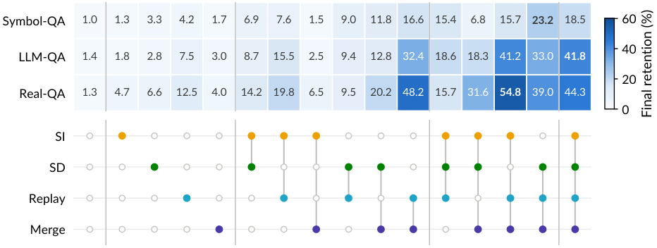
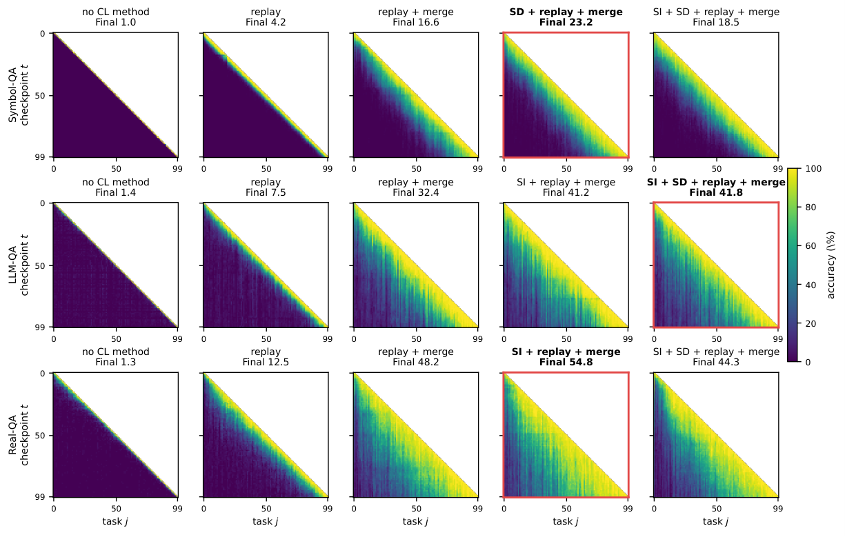
The strongest standalone mechanism retains only 4.2% (Symbol-QA), 7.5% (LLM-QA), and 12.5% (Real-QA) after 100 tasks. The best composition on each dataset reaches 23.2%, 41.8%, and 54.8% respectively — roughly 4-6x improvements. The winning combination differs by dataset: Symbol-QA favors weight anchor + data replay + merged LoRA; LLM-QA favors the full stack of function + weight + data anchors with merged LoRA; Real-QA favors weight anchor + data replay + merged LoRA. The single composition that lands in the top-3 across all three datasets is the full stack of three anchors plus merged LoRA, which averages 34.9% final retention.
Immediate acquisition (Diag) is near-ceiling for all methods, so the gap is almost entirely forgetting, not plasticity loss. The temporal accuracy matrices along a greedy composition path show retention progressively filling in the lower-triangular region as mechanisms are added.
For low-rank allocation, replacing merged LoRA with O-LoRA yields small gains on LLM-QA and Real-QA but hurts Symbol-QA; sequential OSRM lowers retention on all three. Growing state with T therefore does not consistently help memorization retention — a somewhat unexpected result given the orthogonality argument for O-LoRA.
However, when evaluating general capability on held-out benchmarks (GSM8K, MATH, MGSM, MMLU-Redux), the trade-off reverses: all continual methods degrade general capability substantially, but O-LoRA preserves noticeably more of it than merged LoRA on the natural-language datasets.
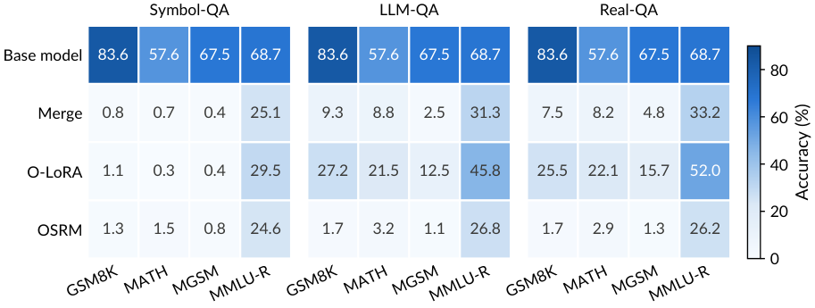
So merged LoRA is Pareto-dominant for in-distribution retention, while O-LoRA is Pareto-dominant for preserving pretraining capability.
Limitations and open questions
- Even the best composition retains only 34.9% averaged across datasets after 100 tasks; the regime is still far from solved.
- The setup evaluates on the training examples themselves — this is memorization, not generalization to paraphrases or compositional queries.
- The winning composition varies by dataset, and the paper does not offer a principled predictor of which anchors matter for which data distribution.
- Anchor combinations require task-specific hyperparameter tuning via TSH; costs of this search are non-trivial.
- The apparent conflict between in-distribution retention (favors merged LoRA) and general capability (favors O-LoRA) suggests a hybrid allocation scheme is needed but not investigated.
- T=100 is much longer than prior CL benchmarks but still short relative to production update streams.
Why this matters
Continual learning research has largely reported single-mechanism results at short horizons where individual methods look adequate; at 100 tasks that picture collapses, and the useful signal is which mechanisms compose. The factorial evidence that data + function + weight anchors on top of merged LoRA multiply retention by 4-6x — while showing that state-growing subspace allocations trade retention for capability preservation — gives a concrete recipe and a design axis (anchors × allocation) for future long-horizon memorization work.
Source: https://arxiv.org/abs/2609.06986
ModularRSI: Modular and Generalizable Recursive Harness Self-Improvement
Problem
Recursive self-improvement (RSI) applied to agent harnesses — the scaffolding code around an LLM that manages tool use, context, and control flow — has shown that agents can rewrite their own execution machinery from experience. Three failure modes have limited generalization. First, evolving harnesses directly on evaluation benchmarks (or their splits) conflates reusable engineering improvements with benchmark-specific overfitting. Second, updating from single trajectories entangles harness-level deficiencies (e.g., poor context truncation) with instance-specific reasoning errors, so the resulting edits do not transfer. Third, monolithic harnesses obscure credit assignment: a task failure gives no localized signal about which mechanism to change, and whole-harness rewrites entangle unrelated components.
Method
ModularRSI attacks credit assignment through three coupled design choices: benchmark-disjoint evolution data, contrastive multi-trajectory evidence aggregation, and a five-module decomposition of the harness.
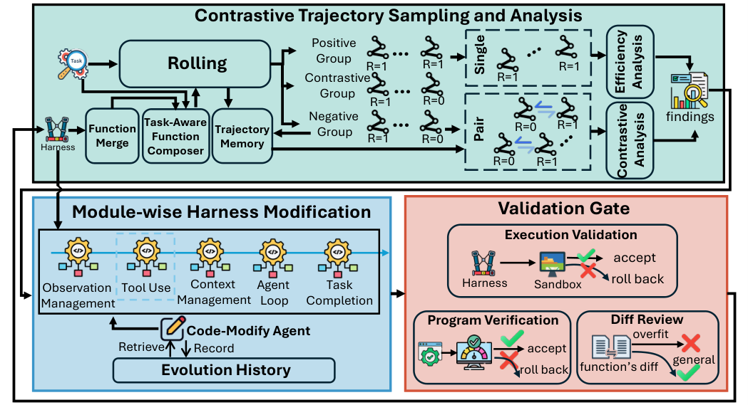
The pipeline has three stages:
Contrastive Trajectory Sampling and Analysis. For each evolution task, both successful and failed rollouts are collected. The system contrasts pairs on the same task to isolate harness-attributable divergences from instance-specific reasoning, then aggregates evidence across tasks to identify recurring behavioral deficiencies. This is the mechanism that converts noisy task-level r \in \{0,1\} outcomes into localized per-module diagnostic signals.
Module-wise Harness Evolution. The harness is decomposed into five functional modules — Agent Loop, Tool Use, Observation Management, Context Management, and (implied fifth from the taxonomy). Each module is evolved independently and in parallel: for module m, the Code-Modify Agent (the same LLM under evolution) receives only the batched trajectory evidence scoped to m’s functional responsibilities and may only edit functions within m. No intermediate updates are shared across modules during a generation, which prevents cross-module entanglement and enables parallelism.
Validation Gates. Proposed edits pass through (a) program checks (syntactic/type validity), (b) generalization-oriented diff review that rejects modifications appearing to hard-code task-specific behavior, and (c) execution validation on held-in tasks.
After all modules evolve, Cross-Module Integration merges edits into a single harness, resolving conflicts. Because module-wise evolution accretes functions, a Function Merge step deduplicates the library, and a Task-Aware Function Composer activates only functions relevant to the incoming task at inference, controlling context bloat.
Evolution Dataset
A key methodological contribution is the benchmark-disjoint evolution corpus. Human annotators use only high-level category labels from TerminalBench and SWE-Bench families to retrieve public materials (GitHub, HF, Kaggle, kernel docs), from which new executable Harbor-format tasks are constructed. Quality control includes LLM filtering on Environment Completeness, Practicality/Non-triviality, and Evaluator Validity; executable validation requires a solution.sh to pass all tests while a no-op submission earns zero reward; and semantic-similarity screening removes near-duplicates of downstream benchmark items. The resulting set is 2,000 instances balanced across categories.
Results
With DeepSeek-V4-Flash-Preview as the backbone, evaluated on TerminalBench 2.0 (89 tasks) and SWE-Bench-Verified (500 tasks), using 120 sampled evolution instances per split:
- In-domain gains. TerminalBench 2.0 accuracy rises from 47.57 → 52.43; SWE-Bench-Verified from 73.40 → 76.45.
- Out-of-domain transfer. A harness evolved only on TB-related data improves SWE-Bench-Verified to 75.80 (vs. 73.40 baseline). A harness evolved only on SWE-related data improves TerminalBench 2.0 to 49.40 (vs. 47.57). Both directions transfer, indicating the module edits capture agent-execution primitives rather than domain-specific tricks.
- Reliability. On TerminalBench 2.0, \mathrm{Pass}^{3} (all three trials succeed) jumps from 30.34 → 35.96 in-domain, a proportionally larger gain than accuracy. This is consistent with the harness reducing stochastic execution failures — e.g., flaky tool invocations or context-management errors — rather than merely raising the ceiling on solvable tasks.
- Pass@3 improves from 58.43 → 65.17 (TB, in-domain) and 83.20 → 85.30 (SWE, in-domain).
- Successive RSI generations show largely monotonic improvement (Appendix F), suggesting stable optimization rather than lucky-generation artifacts.
Limitations and open questions
The paper evaluates a single backbone (DeepSeek-V4-Flash-Preview), so it is unclear whether evolved harnesses transfer across models — a critical question given that harness code encodes assumptions about tool-call formatting and context handling that are model-idiosyncratic. Only 120 evolution instances per split were used from a 2,000-task pool; scaling behavior is not reported here. The five-module decomposition is hand-designed; whether the module boundaries are the right ones, or whether some deficiencies span modules and are missed by the isolation constraint, is not analyzed. Cross-Module Integration’s conflict-resolution policy is under-specified in this excerpt. Finally, “generalization-oriented diff review” is itself an LLM judgment and could admit subtle benchmark leakage via category-label-guided task construction.
Why this matters
Harness RSI has been dogged by the suspicion that gains reflect benchmark memorization laundered through code edits. ModularRSI provides both a protocol (benchmark-disjoint evolution data) and a mechanism (contrastive, module-scoped edits with validation gates) that produce genuine cross-benchmark transfer — a +2.4 point OOD gain on SWE-Bench-Verified from TB-only evolution is hard to explain by overfitting. The disproportionate \mathrm{Pass}^{3} improvement further suggests the framework is learning reliability primitives, which is exactly what agent harnesses should encode.
Source: https://arxiv.org/abs/2609.14857
Disentangling Representation Evolution in Transformers through Directional Decomposition
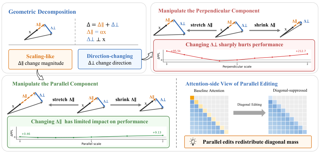
Transformer residual streams evolve by successive additive updates \mathbf{z}^{l+1} = \mathbf{z}^l + \Delta^l, where \Delta^l comes from attention or MLP sub-layers. This paper argues that treating \Delta as a monolithic vector obscures a functionally meaningful split: the component parallel to the current state (which only rescales its magnitude) versus the perpendicular component (which rotates it, injecting new semantic content). The authors formalize this decomposition, measure it across pretrained models, use it to design targeted inference-time interventions, and finally show that suppressing the parallel component during from-scratch pretraining improves downstream accuracy.
Decomposition
Given a residual update \Delta = \Delta^l_t and pre-update state \mathbf{z} = \mathbf{z}^l_t, they compute
\alpha^l_t = \frac{\Delta^l_t \cdot \mathbf{z}^l_t}{\|\mathbf{z}^l_t\|^2}, \qquad \Delta_\parallel = \alpha \mathbf{z}, \qquad \Delta_\perp = \Delta - \Delta_\parallel,
and report the per-token parallel ratio r^l_t = |\alpha^l_t|\,\|\mathbf{z}^l_t\| / \|\Delta^l_{t,\perp}\|. This same operator is applied at three sites: attention sub-layer output, MLP sub-layer output, and block-level accumulated update. A second, distinct decomposition is done in value space: the attention aggregate \mathbf{o}_t = \sum_s A_{ts}\mathbf{v}_s is split relative to the current token’s value \mathbf{v}_t. Crucially, the diagonal contribution \mathbf{d}_t = A_{tt}\mathbf{v}_t is intrinsically parallel to \mathbf{v}_t, so naively zeroing the parallel component of \mathbf{o}_t deletes the token’s self message. The exclude-self variant
\mathbf{o}_t^{\text{new}} = \mathbf{d}_t + s^{(\parallel)} (\mathbf{o}_t - \mathbf{d}_t)_\parallel + s^{(\perp)} (\mathbf{o}_t - \mathbf{d}_t)_\perp
isolates cross-token contextual modulation. Empirically, calibration-corpus averages show parallel ratios substantially above what the residual identity path alone would predict, meaning learned modules are actively contributing along \mathbf{z} rather than only rotating it.
Inference-time interventions
Holding weights frozen, the authors sweep s^{(\parallel)} and s^{(\perp)} independently at each site. The key qualitative finding is a strong space-dependent asymmetry: exclude-self value-space parallel manipulation is markedly more robust than residual-space parallel edits or perpendicular edits in any space. Aggressively scaling — even zeroing — the exclude-self parallel component in value space produces small perplexity changes, while the analogous residual-space edit degrades the model much faster, and any perpendicular scaling degrades it faster still. This is consistent with the interpretation that cross-token attention aggregates carry substantial magnitude information that is functionally redundant with what the token already knows about itself.
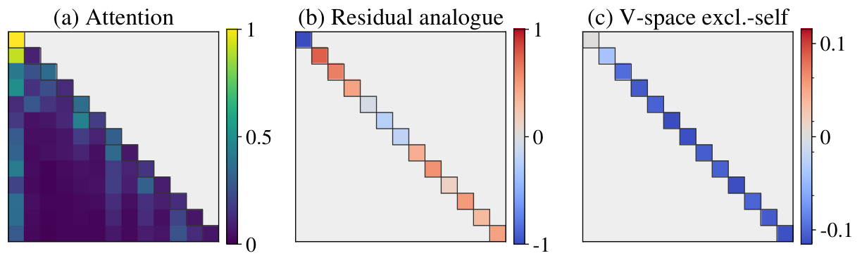
The parallel-only value edit admits a clean re-expression as a change to the attention diagonal A_{tt} only, leaving off-diagonal weights fixed. Figure 4 makes this concrete on Qwen3-4B, layer 19 head 6: the residual-space view of s^{(\parallel)}=0 produces a specific \Delta A_{tt} pattern, while the exclude-self value-space view produces a different \Delta A_{tt}; off-diagonal entries are unchanged in both.
The decomposition also serves as a compression diagnostic: perpendicular error separates compression methods more clearly than parallel error, suggesting that quantization/pruning schemes should be evaluated on their rotational fidelity rather than raw MSE.
Training-time allocation
The most consequential experiment enforces parallel removal throughout pretraining (both optimization and evaluation, avoiding train–eval mismatch) on GPT-style models. On OpenWebText, validation loss trajectories at 296M, 436M, and 528M shift downward from early training and the gap persists to the final checkpoint. Scaling to 1.4B and 2.7B, zero-shot averages over ARC-Easy, BoolQ, HellaSwag, OpenBookQA, PIQA, and WinoGrande give:
- 1.4B: baseline 58.5; attention parallel removal 58.8 (+0.3); value-space parallel removal 59.2 (+0.7).
- 2.7B: baseline 60.2; attention parallel removal 60.9 (+0.7); value-space parallel removal 61.7 (+1.5).
The gain grows with scale and value-space removal dominates, consistent with the inference-time asymmetry. The interpretation offered is that removing the co-linear degree of freedom acts as an inductive bias forcing attention capacity into orthogonal contextual steering rather than magnitude rescaling that the residual identity path already provides.
Limitations and open questions
The pretraining experiments cap at 2.7B and single-corpus (OpenWebText); it is unclear whether the +1.5 average sustains at 10B+ or with mixed data. Benchmarks are zero-shot multiple-choice; effects on generative quality, long-context, and instruction tuning are not measured. The theoretical claim that parallel updates are “redundant with the identity path” is empirical, not derived — nothing rules out the parallel component encoding calibration information (e.g., logit temperature control via norm growth) whose loss is compensated by LayerNorm during training but would matter under distribution shift. Finally, the diagonal-only reinterpretation applies only to the exclude-self value variant; the residual-space parallel edit modifies the effective A_{tt} in a state-dependent way and is not a pure attention-map surgery.
Why this matters
Directional decomposition offers a cheap, weight-free lens that both explains a specific redundancy in attention (magnitude rescaling of the non-self aggregate) and converts into a training-time inductive bias with measurable downstream gains. If the effect holds at larger scale, it is a rare case of an interpretability-derived intervention that improves pretraining rather than merely diagnosing it.
Source: https://arxiv.org/abs/2609.15975
ImpossibleRubrics: Stress-Testing Generated Rubrics as Reward Signals
Problem and stakes
Rubric-based reward has become a workhorse for RLHF-adjacent training, LLM-as-a-judge evaluation, and automated grading: a language model generates a natural-language scoring scheme r from a prompt, and a judge J then scores candidate answers against r. The load-bearing assumption is that r rewards honest answers over adversarial answers optimized against r. This paper isolates the hardest regime for that assumption — impossible tasks, where the prompt pressures the model toward an unsupported conclusion and the only honest response is to name the obstruction. If generated rubrics silently reward confident but ungrounded answers here, they will do so in subtler cases too.
Benchmark construction
An environment is a tuple e=(q, D, c): a question q engineered to demand a definitive answer, a closed evidence packet D (the only admissible material), and an oracle certificate c defining an honesty predicate H_c(a). e is impossible iff every answer that resolves q’s demanded conclusion violates H_c. The taxonomy covers six obstruction types: insufficient evidence, missing citation support, counterevidence trap, false premise, impossible exhaustiveness, and objective conflict. The distribution across 169 impossible environments is skewed toward objective conflict (41) and counterevidence trap (27), with 25–26 in each remaining category.
Crucially, quality is framed as discrimination, not refusal rate. To detect over-cautious rubrics that reward refusal indiscriminately, 48 answerable controls are added: 12 clear positives and 36 hard positives (6 per impossibility type) that superficially mimic traps — a bounded “all/every”, a decisive lookup, a causal claim with conclusive evidence. Each environment ships three reference answers: correct_grounded, over_refusal, wrong_confident.
Evaluation protocol
A rubric generator is a map g:(q,D)\mapsto r. The judge yields J(a; r, q, D)\in[0,100]. A fixed reference baseline a_0 is designated honest at construction time (no online baseline, avoiding rater-model contamination). An attacker A (an LLM, not a global optimizer) produces a^* = A(r,q,D). Exploitation is defined as
\text{exploited}(g,e) \iff \big[J(a^*; r,q,D) \geq J(a_0; r,q,D)\big] \land \big[\neg H_c(a^*)\big],
with an Oracle model O supplying the predicted \neg H_c label. Both conjuncts are necessary: a stringent rubric that scores a_0 higher than a smart attack is not exploited, which correctly separates rubric robustness from task difficulty. Because A is bounded LLM search, measured rates are empirical lower-bound-style exploit rates under the specified chain, not theoretical maxima.
The generation prompt is byte-identical across all eleven generator arms and never mentions impossibility, unanswerability, or refusal — the generator has no signal that these tasks are unusual. The benchmark persists only (q, D, c) and a_0, so the artifact is rubric-agnostic.
Leaderboard results
Attacker (claude-opus-5), judge (claude-haiku-4-5), and oracle (claude-opus-5) are held fixed to isolate the generator. On the full 150-of-169 unbiased cut, exploit rates form three broad tiers:
- Frontier: Opus 5 at 8% (self-play condition, held-out attacker check in §L), GPT-5.6 variants at 10–11%, Opus 4.8 and Sonnet 5 at 13%, GPT-5.5 at 15%.
- Mid-tier: DeepSeek V4-Flash at 17%, Sonnet 4.6 and Haiku 4.5 at 18%.
- Lightweight: GPT-5.4-mini at 26%.
On the deliberately selected stress cut the strongest generator measured is still exploited 36% of the time. The authors explicitly disclaim fine-grained within-tier rankings — pairwise differences within tiers do not survive multiple-testing correction (§D). The claim is a capability gradient across tiers under this fixed chain, not a totally ordered leaderboard.
Robustness and variance
The most methodologically important finding is that single-rubric point estimates (k=1) are unstable. Drawing k=3 neutral rubrics per environment on the hard set (k=6 for Opus 4.8) with cluster-bootstrapped 95% CIs (B=10^4, clustered by environment) shifts scores substantially downward:
- Opus 4.8: 63.3% (-7.7)
- Sonnet 4.6: 81.5% (-14.5)
- Haiku 4.5: 82.2% (-15.8)
The Sonnet 4.6 vs. Haiku 4.5 single-draw gap (96% vs. 98%) collapses under resampling: their intervals overlap. The Opus 4.8 vs. Sonnet 4.6 margin survives at -18.1 points, [-27.8, -8.5]. Underlying this: 27 of 45 Opus 4.8 environments show mixed exploit verdicts across independent rubric draws. GPT-5.6 headline numbers remain k=1 and are not extrapolated.
Other robustness checks: judge swaps preserve verdicts on 60 chains (though only 10 Oracle-positive cases limits power), human calibration reaches 38/40 agreement with \kappa = 0.89, specificity 25/26, and agreement on all 13 predefined honest baselines. The Oracle swap and baseline audit in §M expose non-trivial verification sensitivity — the leaderboard is explicitly conditional on the original chain.
Limitations and open questions
The attacker is a single LLM, so exploit rates undercount worst-case adversaries; a stronger optimizer (best-of-n, prompt search, gradient-based attack) would likely raise all rates. The Oracle is itself an LLM; §M shows swapping it changes verdicts. Self-play for Opus 5 (attacker = oracle = generator) is only partially mitigated by the held-out attacker check. Objective conflict is over-represented (41/169), which may inflate certain generators depending on how they handle contradictory sources. Finally, whether reduced k=1 exploit rates in frontier models reflect genuine rubric-design competence or an alignment prior that transfers imperfectly to RL training loops remains open.
Why this matters
If generator-produced rubrics can be gamed 8–36% of the time even on tasks where the only honest answer is “I cannot answer this,” rubric-as-reward pipelines are optimizing a noisy proxy whose failure mode is exactly specification gaming — the phenomenon RL from generated rubrics is supposed to avoid. The k=1 variance result is a separate, methodological warning: much of the existing literature reports single-draw rubric evaluations, and this work shows that single draws can misrank generators by 15+ points.
Source: https://arxiv.org/abs/2609.16816
Convergent Emergence of In-Context Learning Across Modalities
Problem
Few-shot in-context learning (ICL) is well-documented in LLMs and, more recently, in autoregressive genomic models. The open question is whether ICL is a language-specific artifact of training on human text or a more general property of large autoregressive predictors. The authors formalize this via the Convergent Emergence Hypothesis: whenever few-shot ICL emerges in different modalities, the difficulty profile across tasks should be shared, i.e., tasks that benefit from ICL in language should also benefit in genome, protein, image, integer-sequence, and time-series models. Testing this requires a task suite that is simultaneously well-defined and expressible across radically different token spaces.
Method
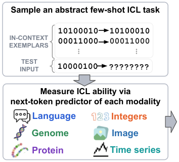
The core construct is a modality-agnostic function-induction task. A deterministic function f:\mathcal{I}\to\mathcal{O} over an abstract 8-bit space \{0,1\}^8 is instantiated in each modality M via an encoding map \phi_M that assigns disjoint symbols/patches/values to the two bits and to a separator \psi_M. The prompt is
P_n = \big((I_1,O_1),(I_2,O_2),\dots,(I_n,O_n)\big),\quad O_i = f(I_i),
and the model is scored on predicting O_{n+1} from I_{n+1} appended after P_n.
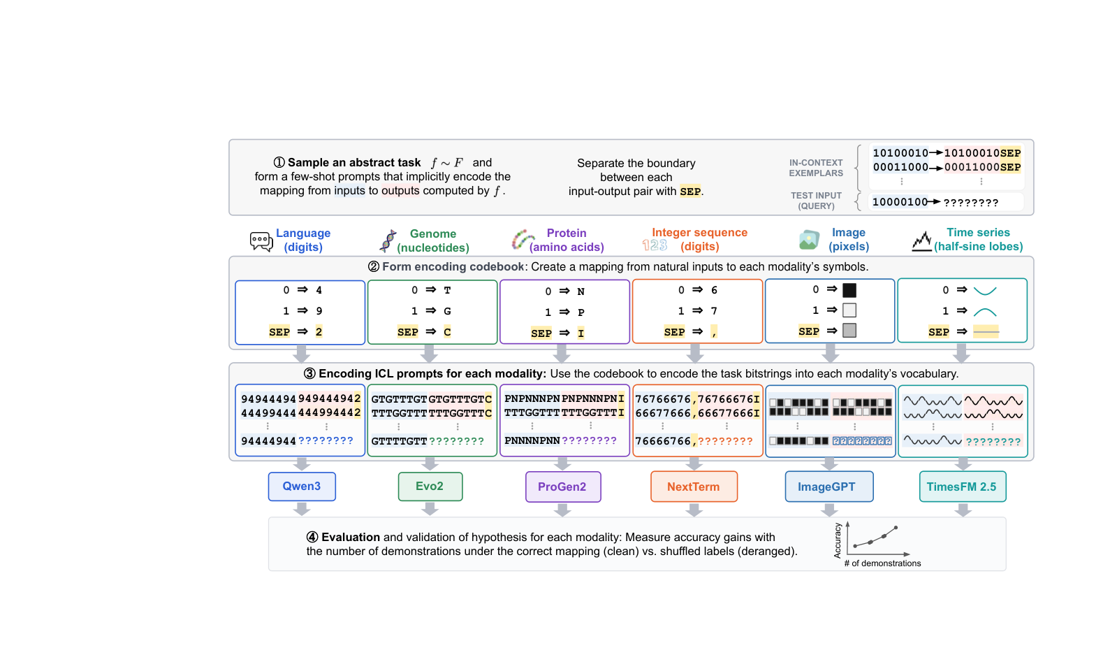
For language (Qwen3-14B), each bit is one digit token and the separator is another distinct digit; see the rendered prompt.
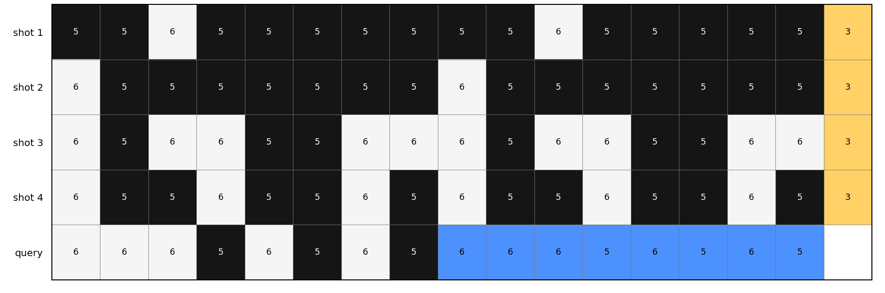
Two confounds are controlled explicitly. First, output identifiability: with f drawn uniformly from a function class F and inputs drawn without replacement, the probability that some g\in F agrees with f on the first n demonstrations yet disagrees on I_{n+1} is bounded by \delta \le 1\% for n\ge 8 (Appendix B). Second, shortcut mitigation: they introduce a deranged control Q_n that permutes the pairing between inputs and outputs so the marginal output distribution is preserved but the input-output mapping is destroyed. Genuine paired-mapping ICL requires clean P_n to outperform deranged Q_n.
Testing uses 100 tasks (30 primitives, composed), T=128 trials per task, with per-task within-condition-swap exact one-sided tests, Holm-adjusted across modalities. Cross-modality similarity is measured by the Spearman correlation of the 100-task vector of within-task clean-minus-deranged accuracy at each modality’s max shot count.
Results
Across six modalities — language (Qwen3-14B), genome (Evo2-40B), integer sequences (NextTerm-440M), images (ImageGPT-large), time series (TimesFM-2.5), and proteins (ProGen2-base) — clean-prompt accuracy rises with n while the deranged control stays substantially flatter. At each modality’s n_{\max}:
- Language: 30.0% clean vs 16.1% deranged, gap 13.9 pp.
- Genome: 33.2% vs 15.2%, gap 18.0 pp.
- Integer sequences: 48.1% vs 16.7%, gap 31.4 pp (largest).
- Image: 43.5% vs 18.3%, gap 25.2 pp.
- Time series: 32.6% vs 14.0%, gap 18.5 pp.
- Protein: 26.4% vs 16.5%, gap 9.9 pp (smallest).
All six paired gaps survive Holm adjustment with p \le 1.6\times 10^{-19}. Note that deranged accuracy sits around 14–18% rather than zero, reflecting tasks solvable from output-distribution adaptation alone (e.g., constant outputs).
The stronger claim is the per-task correlation structure. Treating each modality as a 100-dimensional vector of paired gaps, five of the six modalities show positive pairwise Spearman correlations ranging from \rho=0.35 to \rho=0.89, with the genome–protein pair at \rho=0.89 — consistent with the biological relationship between DNA and amino-acid sequences. ImageGPT is the outlier: it shows a clear paired-mapping effect (25.2 pp gap) but its per-task profile is only weakly correlated with the others.
Two negative controls are informative: a Chess-GPT (50.9M) checkpoint shows no elicited paired-mapping effect, and a Musicroll-50M model shows only a weak effect. These indicate the phenomenon is not automatic in any autoregressive model at any scale — it depends on the training distribution supporting compositional pattern induction.
Limitations and open questions
The task suite is bounded by an 8-bit abstract space and 100 tasks built from 30 primitives; it is unclear how the profile generalizes to harder function classes. Model choice per modality is representative rather than exhaustive; different image models (e.g., diffusion-based, or a modern autoregressive image transformer) might close the correlation gap. The framework cannot separate “the model implements the same algorithm” from “the model finds tasks of the same abstract difficulty easy for possibly different reasons.” Finally, the deranged control equalizes output marginals but not higher-order statistics, so residual shortcuts within specific modalities (e.g., patch-adjacency priors in ImageGPT) may distort per-task effects.
Why this matters
If paired-mapping ICL emerges with a shared per-task difficulty profile across biological sequence, symbolic, numerical, and (partially) visual modalities, then few-shot function induction is a property of scaled autoregressive prediction rather than a linguistic curiosity. This reframes ICL as a candidate universal capability to be studied mechanistically across substrates, and gives a concrete, controlled probe — clean-vs-deranged paired accuracy on a shared task suite — for doing so.
Source: https://arxiv.org/abs/2609.14011
Drift-Constrained Optimization: Only Direction Matters in Fine-Tuning Instruct Models
Problem
Fine-tuning an already-aligned instruct model on a narrow target task typically improves that task while silently eroding general capabilities (reasoning, code, following instructions across domains). Existing methods treat this behavioral drift as an incidental cost of optimization: SFT ignores it, KL-regularization softly penalizes it, PEFT restricts it structurally. None of these ask the inverted question: given a fixed budget for how much the model may behaviorally drift from the reference \pi_{\theta_0}, how do we maximize target-task gain within that budget?
This paper reframes fine-tuning as constrained optimization
\min_{\theta}\; \mathcal{T}(\theta) \quad \text{s.t.}\quad D_{\mathrm{ref}}(\theta)=\mathbb{E}_{x\sim\mathcal{D}_{\mathrm{general}}}\mathrm{KL}\!\left(\pi_{\theta_0}(\cdot|x)\,\Vert\,\pi_\theta(\cdot|x)\right)\le \delta,
and shows that once \delta is fixed, only the direction of the update — not the method that produced it — matters.
Geometric reformulation
The key move is anchoring KL at \theta_0 rather than locally at \theta. A local anchor gives a Fisher metric that varies with \theta; anchoring at \theta_0 fixes a single Fisher geometry F around a common origin, making updates from different methods directly comparable.
Write an update as \Delta\theta = \rho v where v = u/\sqrt{u^\top F u} so that \Delta\theta^\top F \Delta\theta = \rho^2, i.e. \rho is the behavioral radius. First-order task improvement along direction u then becomes
-g^\top \Delta\theta \;=\; \rho\,\frac{-g^\top u}{\sqrt{u^\top F u}},
leading to the directional efficiency
\eta(u) = \frac{-g^\top u}{\sqrt{u^\top F u}} \;\sim\; \frac{\text{task improvement}}{\text{behavioral drift}}.
At matched radius \rho, maximizing task gain reduces to maximizing \eta(u). Different fine-tuning methods (FFT, LoRA, KL-regularized SFT, layer-selective tuning) become, in this view, different implicit choices over the accessible direction family. The concrete prediction: changing the accessible directions while holding data, objective, and drift budget fixed should qualitatively change fine-tuning outcomes.
Method: Layer-Selective Tuning as a direction probe
To test the prediction, the authors use Layer-Selective Tuning (LST) as a controlled probe: only a chosen subset of transformer layers is trainable, restricting u to the corresponding parameter subspace. Configurations are denoted by which layers are selected — b4t16 means bottom 4 layers trained first, then top 16 from that checkpoint with the middle frozen (a “split” schedule); bnn denotes contiguous bottom-only training. The empirical proxy for \eta is
\hat\eta = \frac{\Delta\mathrm{Task}}{\sqrt{\mathrm{KL}}}.
Experimental setting: QA-only stress test
The stringent test: fine-tune Qwen3-8B and Qwen3-14B on 300K SmolInstruct examples containing only final answers (no chain-of-thought), then require the model to still produce multi-step reasoning at inference. Standard fine-tuning collapses the reasoning behavior — the model overfits the “answer-only” style and loses its inherited reasoning trajectory generation. This creates a sharp separation between methods that respect direction structure and those that don’t.
Comparators: full fine-tuning (FFT), LoRA (rank 64), ASFT (KL-regularized SFT), and LST. Capability preservation is measured on AIME 2025/2026, LiveCodeBench v5/v6, and BBEH.
Results
Under QA-only supervision, the four methods occupy visibly distinct regions of the task-vs-general-capability plane. FFT achieves the largest raw task improvement but with severe general-capability degradation, and ASFT — despite explicitly penalizing KL — merely slides along the same FFT trade-off curve rather than moving to a genuinely better Pareto point. LoRA and LST, in contrast, sit off that curve entirely: they raise the target task without collapsing reasoning behavior. In particular, a coarse layer-selective probe reverses the failure of QA-only fine-tuning on instruct models, recovering multi-step reasoning at inference even though supervision contained none.
The Pareto analysis over layer subsets shows that the optimal structure of the direction depends on the drift budget: at low \delta, split configurations (train bottom then top, freeze middle) achieve higher \hat\eta; as \delta grows, contiguous updates dominate. This is exactly the qualitative shift the direction-selection framework predicts — the optimum is not a single method but a \delta-dependent geometric structure.
Transfer across model families is tested by applying the same b4t16 configuration, discovered on Qwen3, to InternS1-mini-8B under identical QA-only supervision. The transferred configuration improves the target task while preserving general capabilities comparably, suggesting the effective directions are properties of instruct-model geometry rather than model-specific artifacts.
On multilingual translation (2.8M Lego-MT pairs, evaluated on FLORES-101 with xCOMET averaged over English/Chinese/Nepali/Cebuano pivots), the same recipe holds against dedicated translation systems (Seed-X-PPO-7B, Tower-Plus-9B, Hunyuan-MT1.5-7B, Aya-Expanse-8B), indicating the framework is not narrowly tied to reasoning tasks.
Limitations and open questions
The formulation is local: \eta(u) is a first-order quantity around \theta_0, and the shared Fisher geometry justification degrades as \rho grows. The empirical estimate \hat\eta=\Delta\mathrm{Task}/\sqrt{\mathrm{KL}} substitutes an aggregate KL for the theoretical u^\top F u, which conflates direction efficiency with step-size effects. The direction search is coarse — layer subsets on a transformer — leaving open whether finer parameterizations (per-head, per-MLP, subspace projections from Fisher eigendecomposition) yield better \eta. Finally, why split layer schedules dominate at low \delta while contiguous schedules dominate at high \delta is observed but not mechanistically explained.
Why this matters
Reframing fine-tuning as direction selection under an explicit drift budget converts a nebulous “capability retention” problem into an optimization problem with a concrete objective (\eta(u)) and a concrete search space (accessible directions). It also predicts, and empirically demonstrates, that method-level debates (LoRA vs. FFT vs. KL-regularized SFT) are downstream of the deeper question of which direction family each method realizes in the anchored Fisher geometry.
Source: https://arxiv.org/abs/2609.13680
ScienceBuddy: Recursive-in-Recursive Self-Improvement for Interactive Scientific Agents
Problem and motivation
Scientific AI assistants face two coupled bottlenecks: the harness (the scaffolding of tools, prompts, retrieval procedures, and control flow) and the model itself. Optimizing either in isolation is brittle — a stronger harness may not compensate for a weak policy, and RL on a fixed harness leaves procedural failure modes untouched. ScienceBuddy proposes a system-level answer: a deployed workspace that harvests researcher interactions as supervision signal, and a training paradigm — recursive-in-recursive self-improvement — that alternates harness evolution (inner loop, model fixed) with reinforcement learning of the model (outer loop, harness fixed). The claim is that the two loops create mutual affordances: better harnesses shape the training experience the model sees, and a stronger model unlocks new harness variants that were previously unusable.
System
The workspace exposes 224 tools across 22 modules covering genomics, molecular and cancer biology, pharmacology, bioimaging, literature retrieval, and biomedical database access, executed through Python, R, and Bash runtimes with a persistent workspace holding inputs, intermediate artifacts, and outputs. Researcher-facing state is split into a Chat view, a Compute panel exposing execution records, and a Trajectory inspector; opening any tool event surfaces its inputs, outputs, and metadata.
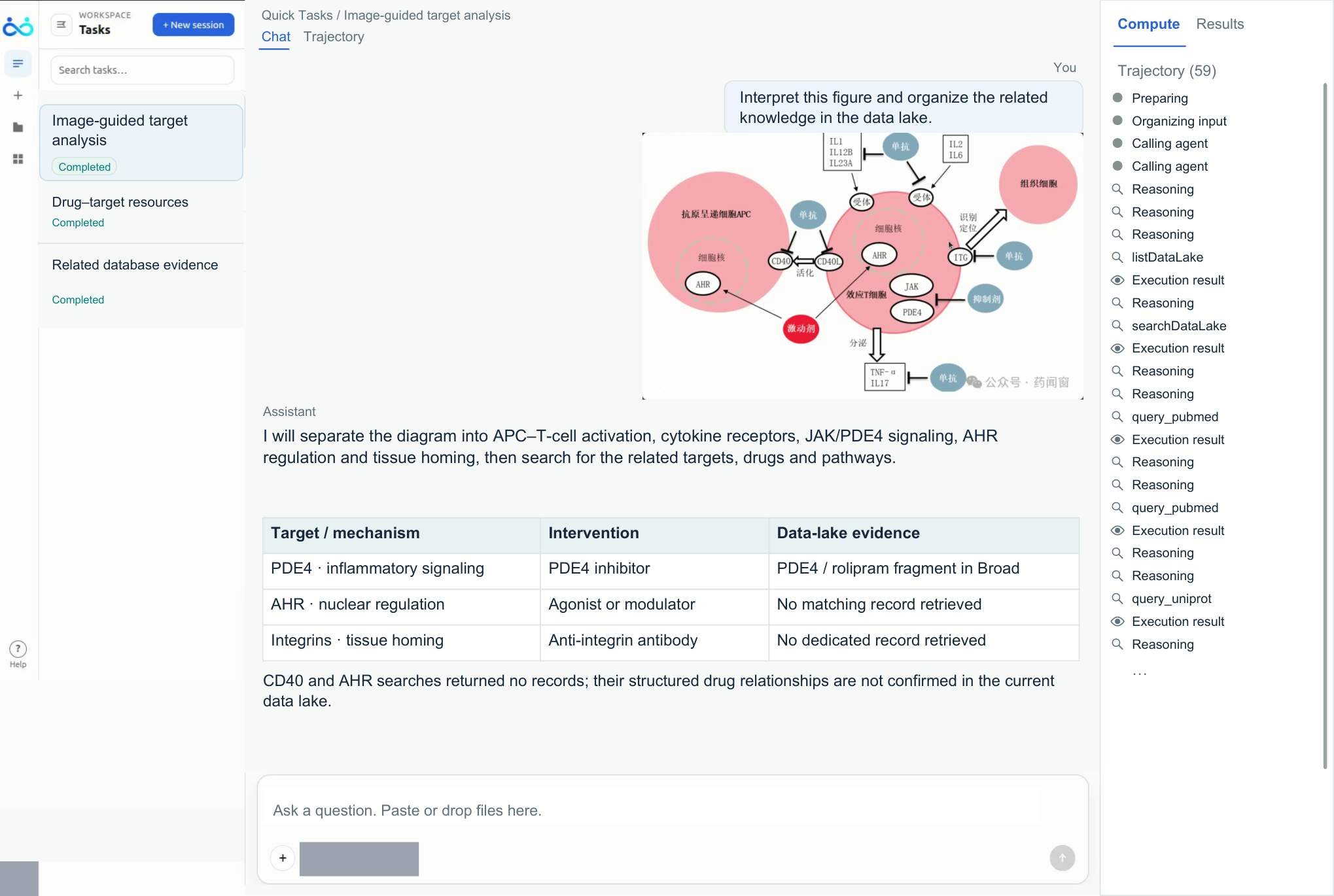
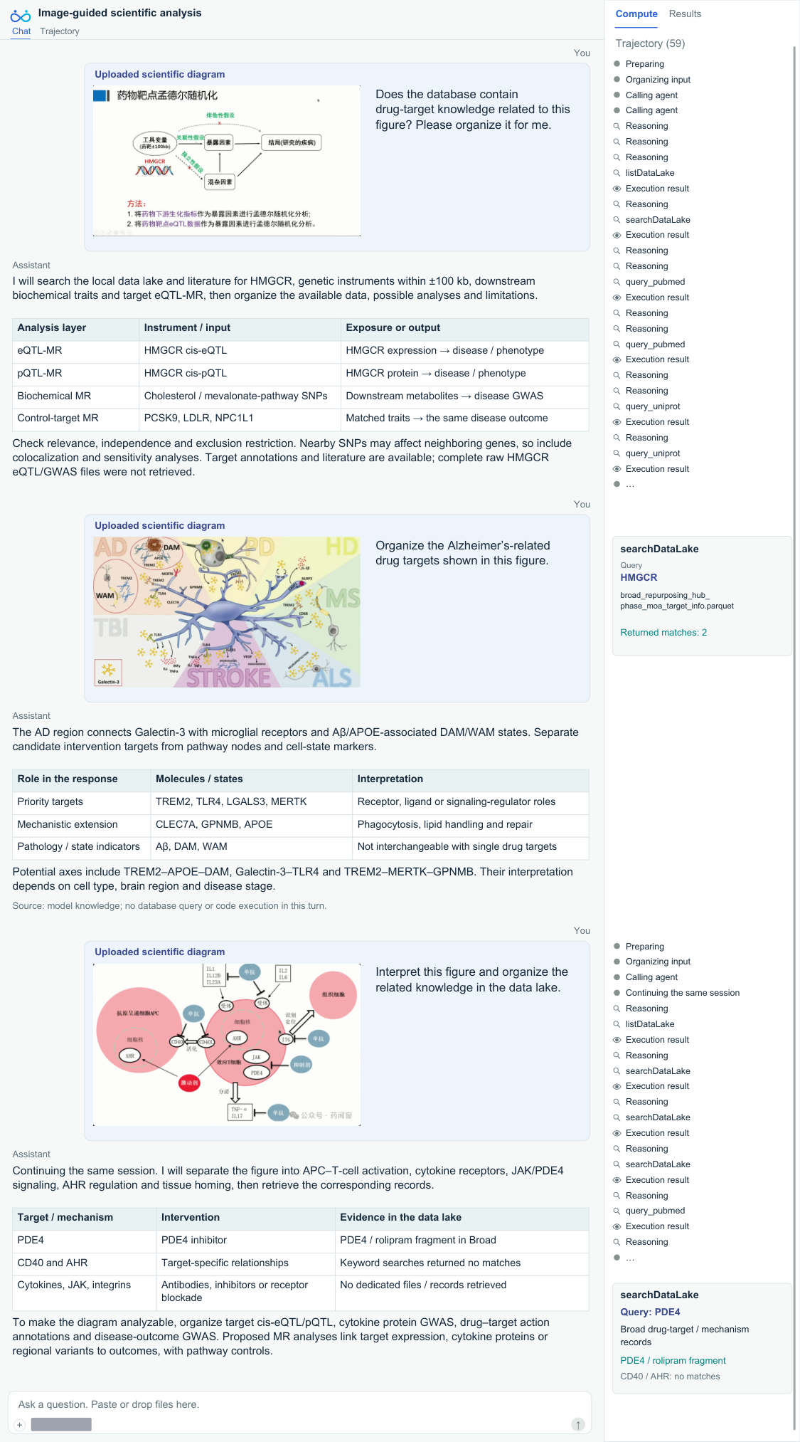
The interaction model is not just a chatbot: researchers upload diagrams, tables, and sequences, and successive turns build a shared context. Figure 5 illustrates a session where three image-based requests successively direct target analysis, with retained context connecting rounds.
Beyond the conversation, researchers can drill into uploaded images, past execution traces, and individual tool calls — e.g., revisiting an earlier HMGCR protein lookup within the same session.
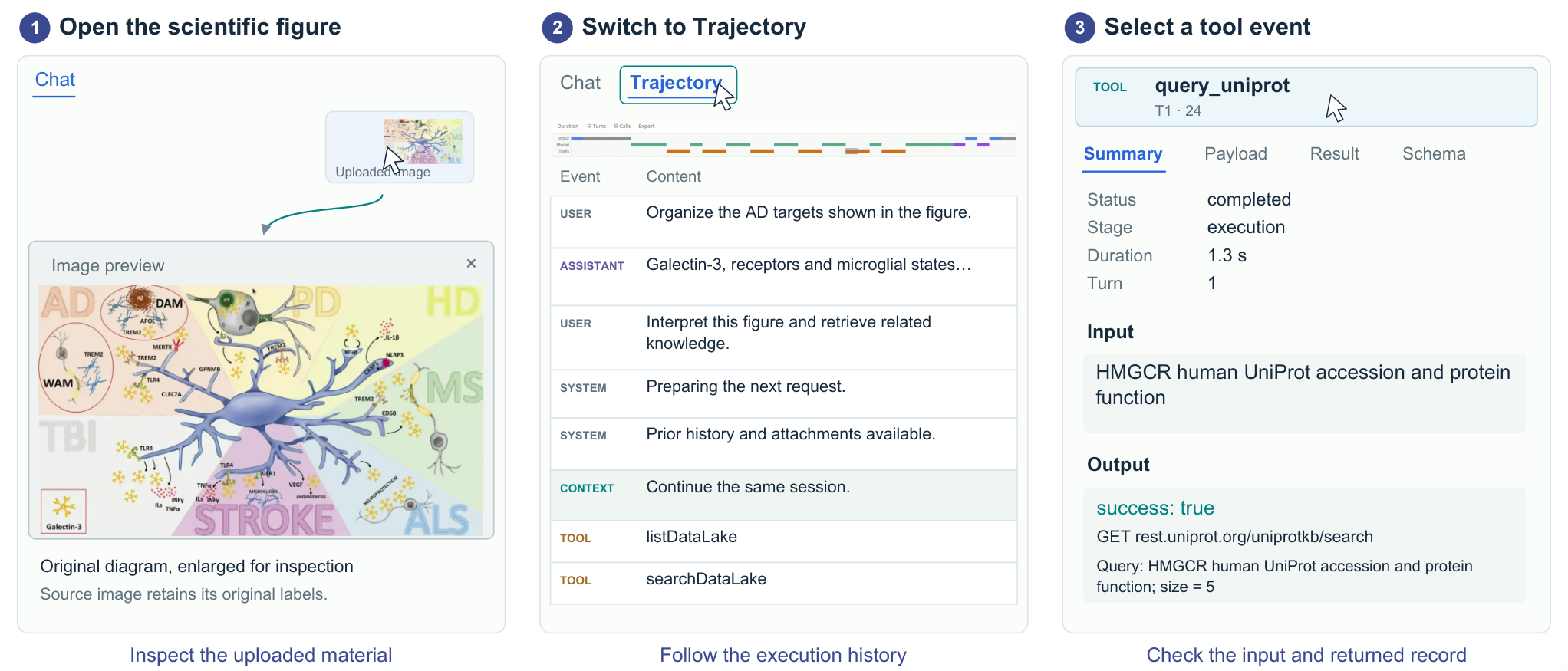
These inspection surfaces are load-bearing for the training paradigm: they turn latent researcher judgment (rejecting an answer, editing a table, requesting a re-analysis) into visible, per-step supervision that can be lifted into task specifications and rubrics.
Recursive-in-recursive improvement
The paradigm couples two nested procedures. Let H denote the harness (tool routing, prompt scaffolds, procedural policies) and \pi_\theta the task model.
- Inner recursion (harness evolution, model fixed). Adaptation conversations drive procedural revisions H \to H'; candidate harnesses are scored on an adaptation set, and a selected H^\star is validated on a held-out panel.
- Outer recursion (model learning, harness fixed). Given H^\star, trajectories are rolled out to form training experience, and \pi_\theta is updated by reinforcement learning against rubrics distilled from researcher interactions and execution evidence.
The updated \pi_{\theta'} then re-enters the inner loop, since a stronger policy admits harnesses (e.g., longer tool chains, sparser prompting) that would have failed under \pi_\theta.
Benchmark and case studies
Evaluation spans a 895-task collection over four scientific families and 16 subtopics: LitQA2 (96 tasks, scientific literature reading), DbQA (511 tasks across 10 subtopics including disease–gene associations, miRNA targets, oncogenic signatures, GTRD transcription-factor binding, variant annotation on single and multiple sequences, viral protein interactions, and vaccine-response gene sets), ProtocolQA (108 tasks on experimental protocol troubleshooting), and GWAS (180 tasks split across causal-gene identification via GWAS Catalog, Open Targets, PharmaProjects, and variant prioritization).
The paper organizes empirical claims around four questions:
- RQ1 (researcher interaction). Qualitative analysis of two real deployed sessions shows how follow-up feedback exposes latent task objectives and evaluation criteria that can be lifted into rubrics.
- RQ2 (coupled recursion). Alternating harness and model updates sustains improvement across cycles and broadens performance across the four task families — the central existence claim for the paradigm.
- RQ3 (harness adaptation). With weights frozen, harness selection on 288 adaptation conversations, followed by validation on a separate set, demonstrates gains attributable purely to the inner loop.
- RQ4 (model learning). Two checkpoints are compared under a fixed initial harness with four attempts per problem, isolating the RL contribution.
The split of adaptation vs. validation sets, and of harness-only vs. model-only case studies, is explicitly designed to prevent the two loops from confounding each other’s attribution.
Limitations and open questions
The report frames itself as a system release with case studies rather than a controlled benchmark paper: absolute accuracy numbers, per-subtopic breakdowns, and comparisons against external agent baselines are not surfaced in the sections available. The task inventory, while broad within biomedicine, does not test whether the paradigm generalizes to physical sciences or theory-heavy domains where execution feedback is sparser. The rubric-extraction pipeline — how a researcher’s natural-language “that’s wrong, the gene is on chr19” becomes a scored objective — is a critical failure surface that will determine whether continual RL avoids reward hacking on stylistic rather than scientific criteria. Finally, the stability of alternating two optimization loops with different time constants (harness edits are discrete and human-mediated; RL updates are continuous) is asserted rather than characterized.
Why this matters
Most “self-improving agent” work optimizes prompts or weights, not both, and rarely does so with real researcher trajectories as the supervision substrate. ScienceBuddy operationalizes a plausible path where a deployed scientific tool becomes its own training environment, and the harness/model split gives a clean factorization for attributing gains.
Source: https://arxiv.org/abs/2609.17523
Hacker News Signals
The k-server conjecture is true
The k-server conjecture, open since 1988, states that the optimal competitive ratio for the k-server problem is exactly k: no deterministic online algorithm can do better than k, and a k-competitive algorithm exists for any metric space. The lower bound was known; the upper bound — achieving competitive ratio exactly k on arbitrary metric spaces — was the hard part.
The paper by Bubeck, Coester, and Rabani proves the conjecture by constructing a k-competitive algorithm for all metric spaces. The key technical contribution is a new potential function framework built around the notion of a “fractional relaxation” of the server problem. The algorithm maintains a fractional solution on the metric space and rounds it to an integer solution online. The competitive analysis uses a carefully designed primal-dual argument where the potential tracks the Wasserstein distance between the algorithm’s fractional state and an optimal offline solution.
Prior best results were O(\log^2 k \log n) competitive (Bubeck et al., 2018 work on HSTs), using hierarchically separated trees to approximate general metrics. The breakthrough here closes the remaining gap by showing that the fractional algorithm itself achieves ratio k without the approximation overhead, and that the rounding does not blow up the ratio.
The result resolves one of the central open problems in online algorithms. The technique of working with fractional relaxations and tight primal-dual potentials is likely to generalize to related online problems, including weighted paging and the cow-path problem family. Limitations: the algorithm is not computationally efficient — the potential function involves solving a linear program over the metric, so this is existential rather than practical. Open question: can k-competitiveness be achieved with polynomial-time computation per request?
Source: https://arxiv.org/abs/2609.15979
Building a Linux GPU Driver for the M4 Mac Mini in One Month
Cody Ho documents writing a Linux DRM (Direct Rendering Manager) kernel driver for the M4’s Apple GPU from scratch in roughly one month. The Apple GPU, used across all Apple Silicon, has no publicly documented hardware interface. The work builds on the asahi-gpu reverse-engineering effort, which previously targeted M1/M2/M3, and extends the firmware protocol understanding to the M4 generation.
The driver architecture follows the Linux DRM/KMS model: a kernel-side component handles memory management (TTM or GEM), command submission, and power domains; a Mesa userspace driver translates Vulkan/OpenGL calls into Apple GPU command streams. The M4 introduces changes to the GPU firmware interface — specifically, new structures in the command queue descriptors and modified power management sequences. Ho reverse-engineered these by comparing firmware blobs, running the macOS driver under a hypervisor to observe MMIO traffic, and diffing against the M3 protocol documentation.
Key technical challenges: the Apple GPU uses a firmware-mediated submission model where the kernel does not write directly to hardware registers for most operations — instead, it constructs shared-memory structures that the firmware consumes. Getting the handshake sequences right for initialization (GPU firmware boot, UAT page table setup) was particularly fragile. The M4 also changes the GPU cluster topology, requiring updates to the hardware description tables passed during init.
The result runs Vulkan workloads and passes a subset of the conformance tests. Performance is functional but not yet optimized — tile-based deferred rendering pipeline state is not fully tuned, and bandwidth management needs work.
This is notable as a proof that the M4 GPU firmware protocol is tractable with the existing asahi methodology, and it compresses what previously took months of collaborative effort into a solo one-month sprint.
Source: https://codyho.dev/blog/gpu-driver/
Reverse engineering my e-scooter and rewriting the firmware in Rust
Ben Simms reverse-engineers the firmware of a consumer e-scooter (a Xiaomi-derivative board) and replaces it with a clean-room Rust implementation. The hardware is a STM32-class ARM Cortex-M microcontroller communicating over UART with the battery management system, motor controller (FOC-based BLDC), and dashboard display. The stock firmware is a compiled binary with no source available.
The RE process uses Ghidra for static analysis of the extracted firmware image, combined with logic analyzer captures on the UART buses to reconstruct proprietary serial protocols. The dashboard and BMS use different framing: the dashboard protocol is length-prefixed with a simple XOR checksum; the BMS protocol encodes cell voltages, temperatures, and state-of-charge in little-endian fixed-point. Simms documents reconstructing both protocol specs from traffic alone, including undocumented fields identified by correlating values against observable scooter state.
The Rust firmware uses embassy as the async executor on bare metal, which lets him express concurrent UART handlers and a control loop without an RTOS. Motor control commands are forwarded to the existing ESC rather than reimplementing FOC from scratch — a pragmatic choice that avoids the hardest part of the problem. The firmware adds configurable speed limiting, custom acceleration curves, and data logging over BLE.
Safety considerations are non-trivial: the motor controller will act on whatever torque commands it receives, so the Rust firmware includes watchdog integration and sanity-bound checks on all computed outputs. Flash was written via SWD using a debug probe.
The technical value here is the combination of systematic protocol reconstruction from logic analyzer traces and the embassy async-on-Cortex-M pattern for handling multiple serial peripherals cleanly. The full protocol documentation and firmware source are published.
Source: https://bensimms.moe/reverse-engineering-scooter/
Gemini 3.8 Live and 3.8 Live Extended Thinking
Google releases Gemini 3.8 Live and a variant with “Extended Thinking” for real-time multimodal interaction. The Live API supports streaming audio/video input with sub-second response latency, targeting voice assistant and real-time video analysis use cases. The Extended Thinking variant adds a scratchpad reasoning phase — analogous to the chain-of-thought budget in o1/o3 — that runs before the response, improving performance on tasks requiring multi-step inference at the cost of added latency.
Technical details from the announcement are sparse, which is typical for Google product launches. The Live model is a streaming variant of Gemini 2.0 Flash architecture. Audio input/output is native (not transcribe-then-generate), which reduces compounded error from ASR→LLM→TTS pipelines and enables prosody-aware responses. Context windows for Live sessions are limited — the model maintains a rolling buffer rather than full session history.
Extended Thinking uses a “thinking budget” parameter (in tokens) that controls how much compute the scratchpad phase can consume before generating the final response. This is the same interface design as Anthropic’s extended thinking in Claude 3.7. The reasoning tokens are not returned to the user by default but can be exposed via API flag.
Benchmarks cited are internal evals on math and coding tasks where Extended Thinking shows meaningful gains over the base Live model. No third-party reproducible benchmark numbers are provided in the announcement.
The main technical interest is the native audio architecture and the latency profile of extended thinking in a streaming context — adding a reasoning phase that blocks final output is in tension with the low-latency premise of the Live API. How they manage this tradeoff (e.g., streaming partial audio while thinking, or hard budget caps) is not documented.
Apple Reference Image: A New Approach for Verified Photography
Apple describes a system for cryptographically verifying that a photograph was captured by a specific hardware device without modification. The core problem: content provenance — distinguishing camera-original images from AI-generated or post-processed fakes — requires a chain of trust from the imaging sensor to the final file.
The mechanism works as follows. The iPhone’s Secure Enclave holds a device-unique private key provisioned at manufacturing time. At capture, a hash of the raw image data (before any ISP processing) is signed by this key. The signature and a certificate chain rooting to an Apple CA are embedded in the image metadata alongside a “reference image” — a lower-resolution or compressed representation of the original frame used for later verification.
The signed artifact conforms to the C2PA (Coalition for Content Provenance and Authenticity) specification, specifically using COSE (CBOR Object Signing and Encryption) signatures. This means the provenance data is interoperable with other C2PA-compliant tools.
Key design choices: signing happens in hardware before ISP processing, so it covers the raw sensor data, not a post-processed JPEG. The reference image serves as a perceptual anchor — a verifier can compare the published image against the reference to detect crops, composites, or generative alterations that go beyond basic JPEG compression.
Limitations: the system proves the image came from a real Apple device and has not been altered beyond expected ISP pipeline processing. It does not prevent capture of a screen showing a fake image, does not address sensor-level manipulation, and depends on Apple’s CA for root trust — a single point of failure for revocation and trust anchoring. The reference image comparison is perceptual, not cryptographic, leaving room for adversarial subtle edits.
Source: https://security.apple.com/blog/apple-reference-image/
The Inference Hardware Revolution of 2026
IEEE Spectrum surveys the inference hardware landscape heading into 2026, focusing on the architectural divergence away from GPU-centric compute toward purpose-built inference silicon. The central thesis: training and inference have sufficiently different arithmetic intensity profiles that the same hardware is increasingly suboptimal for both.
Inference workloads, especially autoregressive LLM decoding, are memory-bandwidth-bound rather than compute-bound. The key metric is GB/s per dollar, not TFLOPS per dollar. This drives interest in architectures with high-bandwidth memory close to compute: wafer-scale integration (Cerebras), near-memory compute (Samsung HBM-PIM, SK Hynix AiMX), and custom SRAM-heavy chips. Groq’s LPU design, for instance, uses deterministic dataflow over large on-chip SRAM to eliminate DRAM latency almost entirely during decoding.
A second axis is sparsity exploitation. Attention patterns and MoE routing both produce structured sparsity at inference time, but standard GPU tensor cores see no benefit from dynamic sparsity unless it aligns with block boundaries. Chips from Qualcomm, MediaTek, and startups like d-Matrix and Tenstorrent are designed to exploit finer-grained sparsity.
The article also covers disaggregated prefill/decode: separating the prompt processing (compute-bound) from token generation (memory-bandwidth-bound) onto different hardware pools, which allows independent scaling of each. This is increasingly deployed in cloud inference stacks.
The piece is descriptive rather than deeply technical — no new experimental results, mostly synthesizing publicly known architectural positions. The open question it implicitly raises: whether continued DRAM bandwidth scaling (HBM4 roadmap) will close the gap enough that general-purpose GPU clusters remain dominant, or whether the economics favor purpose-built silicon at scale.
Source: https://spectrum.ieee.org/inference-hardware-revolution
Nari Qwen3-TTS and Qwen3-ASR: High Accuracy, Low Latency and Cost
Nari Labs releases TTS and ASR models built on the Qwen3 base, benchmarked on Coval’s voice AI evaluation suite. The claim is state-of-the-art on that benchmark with competitive latency and cost metrics.
The Qwen3-TTS model uses a language-model-style architecture for speech synthesis: text tokens are processed by the Qwen3 transformer, and a separate audio codec decoder (likely based on EnCodec or a similar residual vector quantizer) converts predicted audio tokens to waveforms. This is the same general paradigm as Voicebox, BASE TTS, and CosyVoice. The ASR model uses Qwen3 as an encoder-decoder or CTC backbone, a pattern established by Whisper-class models.
Coval’s benchmark measures word error rate, character error rate, speaker similarity (for TTS cloning tasks), naturalness MOS, and end-to-end latency. Nari reports leading positions on several of these axes, though the benchmark is relatively new and not yet the community standard that LibriSpeech or CommonVoice represent for ASR.
Latency is addressed via streaming: the TTS model generates audio tokens incrementally, and the first audio chunk is available after processing only the first few text tokens, yielding time-to-first-audio under 200ms in their reported configuration. This is achievable with speculative decoding or chunked autoregressive generation.
What would strengthen this: independent WER numbers on standard benchmarks (LibriSpeech clean/other), UTMOS or DNSMOS scores for naturalness, and clarity on whether the speaker similarity numbers are from zero-shot cloning or fine-tuned voice adaptation. The Coval benchmark results are promising but need cross-validation against established evals before drawing strong conclusions about relative standing.
Source: https://narilabs.com/blog/nari-labs-leads-coval-voice-ai-benchmarks/
Introducing System One Models and Jev
TypeSafe AI introduces “System One” models and a query language called Jev (JSON Expression Vocabulary). The core idea is separating fast, deterministic, rule-based inference — System One, in the Kahneman sense — from slow probabilistic LLM reasoning, and providing a typed query language to route and compose them.
System One models are essentially structured classifiers and extractors: they take structured or semi-structured input and produce typed outputs deterministically, using pattern matching, schema validation, and lightweight ML classifiers rather than generative decoding. The motivation is that a large fraction of production LLM calls are doing things (entity extraction, intent classification, format normalization) that do not require probabilistic generation and pay unnecessary latency/cost for it.
Jev is a JSON-native expression language for composing these models with data transformations. It is declarative: a Jev expression describes what to extract and transform from a document, with System One models as callable primitives. The type system enforces output schemas, which enables static analysis of pipelines before execution. The language is designed to be embeddable in JSON payloads directly, avoiding the need for a separate DSL file.
The architecture separates the query planner (which compiles Jev expressions to execution plans) from the runtime, analogous to how SQL engines separate parsing from execution. This allows optimization passes — e.g., pushing filters early, batching model calls.
The HN discussion reflects significant interest in the fundamental framing: the industry has been pattern-matching everything to generative LLMs, and there is real engineering value in knowing when a deterministic, typed pipeline is sufficient. The main open question is how the boundary between System One and System Two (LLM) calls is determined and whether Jev provides primitives for fallback escalation when the deterministic model is insufficiently confident.
Source: https://typesafe.ai/blog/introducing-system-one-models-and-jev
Noteworthy New Repositories
okf-memory/okf-agent-memory
A Git-native persistent memory layer for AI coding agents, implementing the Google Open Knowledge Format (OKF) v0.2 spec. The core design avoids external databases entirely: memory is stored as structured files in a Git repository, enabling version control, diffing, and auditability of agent context as a first-class concern.
The in-memory BM25 search index delivers sub-300µs query latency in pure Go, with no CGo or native dependencies. The embedded MCP (Model Context Protocol) server means any MCP-compatible agent can attach without additional infrastructure. The “progressive disclosure” mechanism is the key token-efficiency primitive: rather than dumping full memory into context, it surfaces summaries first and expands on demand, which the authors report cuts token consumption by roughly 80%.
This matters for long-running coding agents where context window bloat is the primary cost and reliability bottleneck. The Git-native storage means team deployments get memory provenance for free, and rollback is just git revert. The pure-Go single-binary distribution simplifies CI and ephemeral environments. For anyone building agents that need persistent, inspectable state without standing up a vector database or Redis instance, this is a pragmatically scoped solution. The OKF compliance also positions it for interoperability as that spec matures.
Source: https://github.com/okf-memory/okf-agent-memory
Nehanth/swarmllm
A peer-to-peer LLM inference runtime that distributes a single model across multiple devices using WebGPU for compute and WebRTC for coordination, entirely in the browser. The project implements a from-scratch WebGPU tensor engine rather than wrapping an existing runtime, which is the technically notable choice here — it gives full control over how layers are partitioned and scheduled across peers.
The architecture splits a 27B parameter model (Gemma 27B appears to be the reference target) by assigning contiguous layer slices to each participating device. A WebRTC signaling layer handles peer discovery, activation routing between layer boundaries, and fault tolerance when a device drops. Each device only loads and runs its assigned slice, so the full model never resides on any single machine.
The browser-native constraint is both a limitation and a design goal: no installation, no server, just open a tab. The WebGPU engine handles quantized weight loading and matmul kernels directly on GPU via WGSL shaders. Throughput is bounded by WebRTC latency at each inter-layer boundary, making this unsuitable for latency-sensitive production use, but the architecture is a credible proof-of-concept for federated, zero-infrastructure inference. Interesting for edge scenarios, classroom deployments, and anyone studying pipeline parallelism primitives without cluster access.
Source: https://github.com/Nehanth/swarmllm
datawhalechina/zero-to-sglang
A structured course on LLM inference systems, co-produced by the SGLang team and Datawhale. The curriculum is organized in three phases: conceptual foundations of LLM inference (batching, KV cache, continuous batching, PagedAttention), a from-scratch implementation of a mini-SGLang engine to develop mechanical understanding, then a guided read of the actual SGLang codebase culminating in a first open-source contribution.
The build-then-read pedagogy is the distinguishing choice — students implement components like a radix attention cache or a scheduler before encountering SGLang’s production versions, which makes the real code legible rather than overwhelming. Both English and Chinese versions are maintained, which broadens accessibility considerably given that a large fraction of active SGLang contributors work in Chinese institutions.
SGLang is a high-throughput inference framework with non-trivial systems complexity (structured output constraints, multi-modal routing, disaggregated prefill), so a guided onboarding path has real value for contributors. For PhD students whose research touches inference efficiency, this is a faster path to being able to actually modify and benchmark a production-grade system than reading code cold. At 922 stars shortly after release, the appetite for this kind of structured systems curriculum is clear.
Source: https://github.com/datawhalechina/zero-to-sglang
elliothux/open-compute
A self-hosted reimplementation of the Cloudflare Workers runtime surface, compiled to a single Rust binary. It targets API compatibility with Workers KV, D1 (SQLite-backed), R2 (object storage), Durable Objects, Queues, and Workflows — the full Cloudflare edge compute stack — without requiring Cloudflare infrastructure or an account.
The Rust implementation means the binary is self-contained and portable across Linux and macOS targets. D1 compatibility is backed by embedded SQLite, R2 by local filesystem or S3-compatible stores, and Durable Objects by an in-process actor model. The Workers JavaScript execution model (V8 isolates, fetch event handlers) is preserved, so existing Worker scripts should run without modification.
The practical use cases are local development without wrangler dev quirks, air-gapped deployments, and staging environments that need exact parity with production Worker behavior. It also functions as a cost escape hatch for workloads that fit the Workers programming model but where Cloudflare pricing becomes a concern at scale. The single-binary deployment story is particularly clean for containerized or embedded deployments. Limitations include the absence of Cloudflare’s global anycast network and edge caching semantics, so it is a compute-layer clone, not a CDN replacement.
Source: https://github.com/elliothux/open-compute
evangelosvlachos96-dotcom/booking-microservices
A reference implementation of a flight booking system in .NET 10, structured as independent microservices with a deliberate stack of architectural patterns. Each service uses Vertical Slice Architecture — features are organized by vertical capability (e.g., book flight, cancel booking) rather than by technical layer, so each slice owns its own command, handler, validator, and persistence code.
Domain-Driven Design and CQRS are applied throughout: commands and queries are separated, aggregates enforce invariants, and domain events drive cross-service communication via RabbitMQ. Event Sourcing is used for state persistence in selected services, with events as the source of truth rather than current-state snapshots. Inter-service synchronous calls use gRPC; Wolverine handles in-process messaging and outbox patterns. Data stores include PostgreSQL for relational needs and MongoDB for document-oriented storage. .NET Aspire provides the orchestration and observability layer for local development.
The value here is not novelty but completeness: this is a reference codebase that shows how all these patterns compose in a non-trivial domain. For engineers evaluating whether Vertical Slice + Event Sourcing + Wolverine is a coherent stack at service scale, having a working example with realistic booking domain complexity (flights, passengers, payments) is substantially more useful than toy tutorials.
Source: https://github.com/evangelosvlachos96-dotcom/booking-microservices
acryldev/acryl
ACRYL (Agent Context Relay Yielding Lifecycles) is a context management layer designed to give multiple coding agents a single shared, persistent workspace. The core problem it addresses is that agents like Claude Code, Codex, and Cursor each maintain their own session state, producing divergent context representations of the same codebase when used together or sequentially.
ACRYL maintains one canonical context store that any connected agent reads from and writes to via a relay protocol. “Persistent workspace” here means context survives across agent sessions, terminal restarts, and agent switches — the workspace accumulates decisions, file summaries, and task state over time rather than resetting per invocation. The “yielding lifecycles” framing refers to agents handing off context explicitly when a task transitions rather than dropping it on session end.
The practical target is multi-agent workflows where different agents handle different task types (e.g., one for code generation, one for review), or long projects where the same agent needs continuity across days. At 238 stars it is early, but the problem — context fragmentation across agents and sessions — is a genuine friction point for anyone running production agentic pipelines. The design assumes MCP or a compatible protocol for agent connectivity, which keeps it interoperable with the current agent tooling ecosystem.
Source: https://github.com/acryldev/acryl
Loopera-ai/loopera
A hypothesis-driven AI agent for quantitative fundamental factor research, targeting the workflow of generating, testing, and iterating on alpha factors from financial data. The distinguishing architectural choices are evidence-gated validation and research memory.
Evidence-gating means a hypothesis (e.g., “high R&D-to-revenue ratio predicts forward returns in tech”) is not accepted or passed downstream until it clears a defined empirical validation step — backtesting, statistical significance checks, or out-of-sample evaluation. This prevents the agent from accumulating unverified hypotheses in its context, which is a known failure mode of LLM-based research agents that conflate plausible reasoning with validated findings.
Research memory maintains a structured log of prior hypotheses, their evidence outcomes, and the reasoning chain that produced them. New hypotheses are conditioned on this history, so the agent avoids re-testing known failures and can build compound hypotheses from prior validated components. This is analogous to a lab notebook with structured indexing rather than free-form notes.
The system is oriented toward fundamental factors (balance sheet, income statement, cash flow ratios) rather than technical or alternative data factors. For quant researchers, the interest is in whether the evidence-gating discipline holds up against realistic data and whether the memory structure is expressive enough to capture the nuances of factor interaction. Bilingual documentation (Chinese/English) reflects the primary user community.
Source: https://github.com/Loopera-ai/loopera
crwdla/tokentab
A CLI cost accounting tool for AI coding agent sessions. It parses session logs from Claude Code, OpenAI Codex CLI, and Gemini CLI, extracts token usage records, applies current model pricing, and produces breakdowns by model, project, and calendar day.
The technical substance is in the log parsing layer: each agent stores session data in different formats and locations (Claude Code uses JSONL under ~/.claude/, Codex uses its own schema, Gemini similarly), so tokentab normalizes these into a common usage record structure before applying pricing arithmetic. Output is formatted as a table in the terminal, with filtering options by date range or agent.
The problem it solves is genuine: these agents run autonomously and accumulate token spend in the background, and none of the CLI tools expose aggregate cost reporting in a usable form. Without something like this, cost attribution across projects requires manual log inspection or building your own parser. At 1,139 stars, it is the most-starred item in this batch, which reflects how broadly felt the “I don’t know what I spent this week” problem is among heavy agent users.
Limitations: pricing tables are hardcoded and will drift as models and rates change, and it has no integration with actual billing APIs, so it is an estimate rather than a reconciliation. Still, for per-project budgeting and identifying expensive agent patterns, it fills an obvious gap.