Daily AI Digest — 2026-08-31
arXiv Highlights
DART-SD: Diamond-topology Aware Retrieval and Tuning for Self-Distillation of Multi-Turn Tool-Calling Agents
Problem
Training LLMs as multi-turn tool-calling agents typically involves imitation of full teacher trajectories or trajectory-level RL. For tasks with multiple order-independent sub-goals — e.g., gathering four independent facts before answering — the set of optimal action sequences forms a combinatorial diamond lattice: many permutations of tool calls lead to the same information state. Full-trajectory SFT collapses this lattice onto a single ordering, penalizing valid alternative explorations; GRPO-style RL spreads reward uniformly over the trajectory and misassigns credit for the specific step that caused failure.
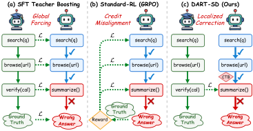
DART-SD replaces global forcing with topology-guided localized correction: identify the exact step at which a failed student rollout leaves the success-reachable region, and only supervise the tokens that follow.
Method
The framework has three components: an Interaction-State Transition Graph (ISTG) built from teacher rollouts, a Critical Topological Breakpoint (CTB) detected by projecting failed student rollouts onto the ISTG, and a localized SFT loss applied only after the CTB.
Information atom abstraction. For task x, tool responses are normalized to a set \mathcal{K}_x of information atoms. A deterministic stage parses each response and collapses non-informative outputs (status signals, empty/placeholder fields, errors) into a per-tool null class. A semantic stage then jointly labels the remaining candidates conditioned on the task question and one successful rollout, producing a set-valued atom map
\alpha_x:\ (\operatorname{tl}(e),\bar{o}(e))\ \longmapsto\ \alpha_x(e)\subseteq \mathcal{K}_x,\ |\alpha_x(e)|\leq 1.
Joint labeling is what makes information-equivalence decidable — the same fact returned as free text by one tool and as a structured record by another is unified into a single atom, so alternative acquisition paths reconverge at the same node rather than forking into artificially distinct states.
Information state dynamics. Let B_t denote the tool-call bundle at step t. The acquisition increment and cumulative information state are
\Delta I_t = \{k \in \mathcal{K}_x \mid \exists e \in B_t,\ k \in \alpha_x(e),\ k \notin I_{t-1}\},\qquad I_t = I_{t-1}\cup \Delta I_t.
Nodes in the ISTG are these information states; main nodes correspond to acquisition-increasing transitions from successful teacher paths, auxiliary nodes model useless exploration observed in failed rollouts. The graph converges: many orderings of B_t land on the same I_t.
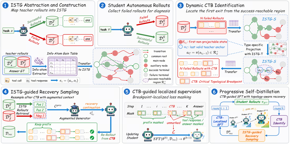
CTB detection. A failed student rollout is replayed step-by-step in the ISTG. Define a budget-filtered success-reachable region \mathcal{R}_x^+: states from which a completing continuation exists within remaining turn/token budget. The CTB is the first index at which the student’s next state is projectable onto \mathcal{R}_x^+ but the step after is not — i.e., the exact transition that leaves the productive region.
Localized self-distillation. The student prefix up to the CTB is retained. Two positive teacher references (with teacher-generated analyses) and one negative reference are appended as privileged context, and the student generates a recovery continuation. SFT loss is masked to apply only to newly generated assistant tokens post-CTB. This loop repeats for 5 iterations over all 2,215 FTRL tasks, 8 rollouts per task, temperature 0.7, up to 9 turns, lr 5\times 10^{-7}, batch size 32, one epoch per iteration.
Results
Teachers are Qwen3.6-27B and GLM-5.2; students are Qwen3-4B and Qwen3-8B; all methods evaluated under a no-thinking configuration. Figure 3 (referenced in the text) reports the Qwen3-8B student improving on all five benchmarks — FTRL (in-domain), BFCL, ToolHop, \tau-bench, RoTBench — and surpassing its own teacher on FTRL, ToolHop, and \tau-bench. Baselines include SFT, SCoRe-SFT, OPSD (distillation) and FTRL-GRPO, ToolRL, MatchTIR-OT/KM (RL). The paper’s abstract/setup emphasizes preserved policy diversity relative to full-trajectory SFT, consistent with the CTB masking design. Specific per-benchmark numerical deltas are not visible in the provided excerpt.
Limitations and open questions
- The semantic atom map \alpha_x relies on an LLM judge conditioned on one successful rollout. If the successful rollout misses a valid alternative fact source, its atoms may be misclassified as null, contaminating the ISTG.
- \mathcal{R}_x^+ is defined by a remaining-turn/token budget; the paper does not analyze sensitivity to this budget. Too tight a budget spuriously advances the CTB; too loose obscures it.
- CTB-localized SFT still uses teacher references as privileged context. It is unclear how much of the gain over standard SFT comes from the loss masking versus from the retrieved reference augmentation (positive+negative+analysis).
- All experiments use FTRL for training; while OOD benchmarks are covered, the atomization procedure may not transfer to environments where tool responses cannot be canonically parsed into fields.
- Comparison to RL baselines under matched compute is not detailed in the excerpt — RL methods have different sample efficiencies that complicate the credit-assignment argument.
Why this matters
Full-trajectory imitation is the standard failure mode when scaling tool-calling agents to real workflows with commutative sub-goals: it destroys the very solution diversity that makes agents robust. DART-SD offers a concrete procedure — atom-based state abstraction, success-reachable projection, and loss masking to a single detected breakpoint — for aligning the granularity of supervision with the topology of the task, and demonstrates that a student can surpass its teacher on multi-hop tool benchmarks under this discipline.
Source: https://arxiv.org/abs/2608.18524
Beyond Data Scaling: Representation-Centric Continued Pre-training for Vision-Language-Action Models
Scaling robot trajectories is expensive and sparsely covers the physical world, so the marginal utility of yet more embodied data plateaus quickly. VLAct reframes VLA continued pre-training as a representation-shaping problem: under a fixed robot-data budget, how should one supervise a VLM backbone so that action-relevant structure is deposited into features that arbitrary downstream heads can decode? The authors identify two failure modes of naive continued pre-training and propose a recipe that specifically avoids both.
Pilot: action supervision is not head-neutral
The pilot study fixes the backbone to Qwen3-VL-4B and sweeps the action head used during pre-training versus fine-tuning. Two failure modes emerge:
Discrete-token pre-training (FAST) loses fine-grained information. A FAST-pretrained backbone paired with a continuous GR00T head slightly improves over from-scratch GR00T fine-tuning, indicating some transferable structure. But keeping FAST as the fine-tuning head is much worse than continuous fine-tuning, and FAST pre-training does not close this gap. Discretization injects coarse action structure but destroys temporal and amplitude precision needed for manipulation.
Single continuous head (OFT) causes head-specific collapse. On RoboTwin-Clean, OFT pre-training substantially helps when the downstream head is also OFT, but the same backbone underperforms when paired with PI or GR00T heads. Action information is present, but the feature geometry has collapsed toward directions that specifically decode with OFT — a form of representation lock-in that inflates same-head benchmarks while destroying reusability.
The pilot’s conclusion is sharp: strong same-head numbers are not evidence of a transferable backbone. A reusable VLA backbone must preserve fine-grained continuous action information while keeping it decodable by multiple heads.
Method: three representation-centric mechanisms
VLAct performs continued pre-training from a Qwen3-VL-4B initialization with three mechanisms designed to counter the failure modes above:
(1) VLM-prior preservation. The vision encoder and shallow LLM layers are frozen, and captioning data is mixed into the robot-trajectory stream. This prevents catastrophic drift of the semantic prior that dense manipulation supervision would otherwise erode.
(2) Multi-head continuous co-supervision. Rather than committing to one continuous head, VLAct routes the shared backbone through OFT, PI (flow-matching), and GR00T (diffusion-style) heads simultaneously during pre-training. Each head imposes a different inductive bias on the action decoder; forcing the backbone to satisfy all three prevents its geometry from collapsing into any single head’s preferred directions. At fine-tuning time all pre-training heads are discarded and a fresh task-specific head is attached — improvements therefore attribute to the backbone, not to a pre-adapted head.
(3) Partially unified cross-embodiment action layout with wrap-aware loss. Robot data spans DROID, InternA1, RoboCoin, and MolmoAct — different embodiments with different DOFs and action semantics. VLAct uses a shared action-layout slot structure with masked inactive dimensions per embodiment, so that overlapping semantics (e.g., end-effector translation) land in the same slots across embodiments. A wrap-aware loss handles the angular discontinuities in rotational dimensions.
The recipe is deliberately asymmetric: pre-training uses heavy multi-head machinery to shape features; fine-tuning uses the same protocol as each baseline with a freshly initialized head, isolating the backbone contribution.
Results
On LIBERO-Plus — which perturbs cameras, robot states, lighting, backgrounds, noise, object layouts, and instructions — VLAct reaches 82.6% total success. The controlled comparison against Qwen3VL-OFT (same backbone family, same OFT downstream head, same fine-tuning protocol) gives +7.6 points (82.6 vs 75.0), isolating the effect of the pre-training recipe. VLAct also beats Abot-M0 (80.5) by 2.1 points while using only open-source data. The per-dimension breakdown is informative: the largest gains over Qwen3VL-OFT are on Camera (73.9 vs 47.0), Robot (68.4 vs 60.1), Noise (86.0 vs 73.1), and Layout (83.3 vs 79.2) — precisely the axes where visual-spatial representation quality dominates, consistent with the hypothesis that representation-centric pre-training improves feature robustness rather than memorized action patterns. Language, Light, and Background scores are competitive but not the source of the gain, since these depend more on the preserved VLM prior than on action supervision.
On RoboTwin 2.0, VLAct reports 92.5%, surpassing LingBot-VLA and other industrial systems (abstract-level number; per-task breakdown in the paper).
Limitations and open questions
The multi-head co-supervision cost scales linearly with the number of heads, and the paper does not report ablations on which subset of heads is minimally sufficient. The partially unified action layout requires manual per-embodiment slot assignment, which will not scale gracefully to highly heterogeneous morphologies (soft robots, mobile bases, dexterous hands). It is also unclear whether the pilot’s OFT-collapse phenomenon quantitatively generalizes to larger backbones or larger pre-training budgets — the effect might attenuate with scale, in which case the multi-head machinery is mainly a small-scale regularizer. Finally, all evaluation uses standard fine-tuning protocols; the claim of a reusable backbone would be strengthened by few-shot or frozen-backbone probes.
Why this matters
VLAct provides a concrete counterexample to the assumption that VLA progress is bottlenecked by trajectory volume: under a fixed data budget, a representation-centric pre-training objective yields a 7.6-point robustness gain over a matched single-head baseline and beats industrial systems trained with far more compute. The pilot’s identification of head-specific representation collapse is a diagnostic worth internalizing for anyone building VLA foundation models.
Source: https://arxiv.org/abs/2608.27550
Code as Worlds: Agentic Discovery of Executable World Representations for Physical Reasoning
Problem
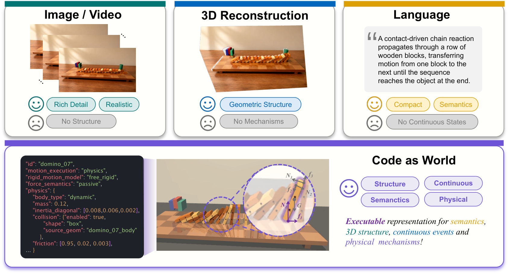
Vision-language models can name physical events but do not maintain the latent variables — mass, velocity, contact state, camera intrinsics — that determine how a scene evolves under intervention. Pixel-space video predictors optimize visual plausibility, which is under-determined: camera motion vs. object motion, occlusion vs. disappearance, and other causally distinct hypotheses can yield indistinguishable next frames. Geometric reconstructions capture shape but not dynamics; language captures semantics but is imprecise about continuous state. The paper argues these three representational families (pixels, 3D, language) individually fail to support compositional, quantitatively grounded physical reasoning.
Method: Code as Executable World Representation
Code-as-World represents a scene as an executable program that specifies (i) physical composition (entities, parameters, relations), (ii) dynamic evolution (governing rules, forces, events), and (iii) visual appearance (materials, lighting, camera). Execution plus rendering yields observations; the criterion of correctness is physical equivalence — matching composition, constraints, and evolution — rather than pixel matching. This factorization separates structured state (compositional, editable, constrained) from continuous appearance (rich but uncertain), which is precisely the split needed for interventional reasoning: one can edit code and re-simulate to obtain counterfactuals.
Recovering an executable world representation (EWR) from a text prompt or real video is under-constrained, so the authors frame it as abductive search. Given input \xi from modality m, a modality-specific adapter produces evidence \eta — structured semantic constraints from text, or visual constraints (trajectories, contacts, camera cues) from video. A shared agent then runs a propose–instantiate–execute–render–verify loop:
- Propose an EWR hypothesis consistent with \eta and physical priors.
- Instantiate parameters (masses, geometries, initial conditions, camera).
- Execute the simulator to produce state trajectories.
- Render frames.
- Verify against \eta: semantic checks for text evidence, trajectory/appearance checks for video evidence.
- Refine and iterate.
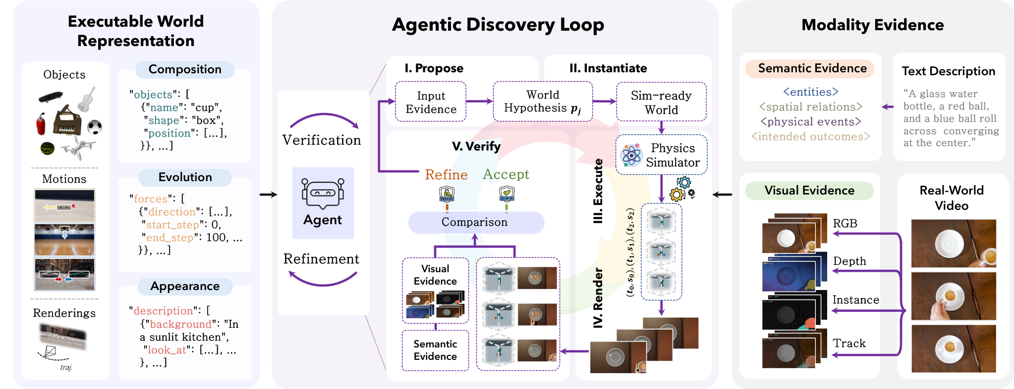
Text inputs are typically incomplete about geometry and physical parameters, so the agent fills them with physical priors and refines through simulation. For visual realism in downstream data generation, verified simulator rollouts are passed through a sim-to-real video generator, which enriches materials, backgrounds, and lighting while preserving the underlying physical trajectory — the state remains the ground truth even as pixels are stylized.
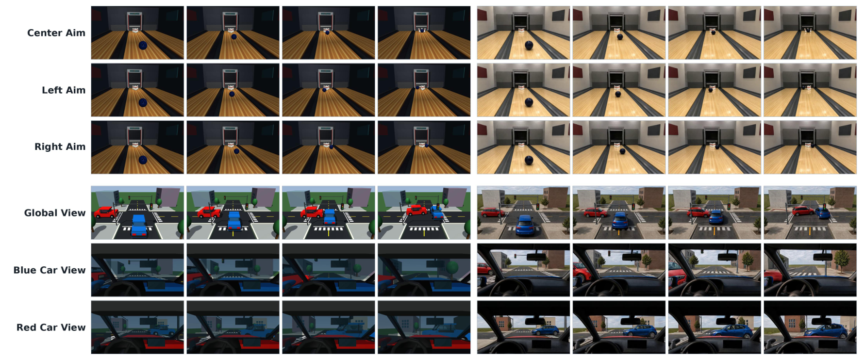
The resimulation figure is the operational payoff: because the world is code, one can edit initial conditions or parameters, re-execute, and obtain a paired (simulator, photoreal) sequence whose physical quantities are known exactly.
Application: Quantitative Physical Reasoning Supervision
The concrete use case is training VLMs to answer quantitative physical questions from monocular video — e.g., real-world size, velocity, or acceleration of a specified object at specified timestamps. The output is \hat{y}=f_\theta(V,q)\in\mathbb{R}. Real videos lack such annotations, so supervision is the bottleneck; Code-as-World supplies it directly from verified EWRs.
Following the QuantiPhy formulation, world-space queries include a reference quantity with known value \rho to fix the metric scale. Given pixel-space measurements y^{\mathrm{pix}} and \rho^{\mathrm{pix}}, the relative scale is
\gamma = \frac{\rho}{\rho^{\mathrm{pix}}},\qquad y = \gamma\, y^{\mathrm{pix}},
and the same \gamma converts pixel displacements, velocities, and accelerations into world units. In 3D settings, monocular depth cues augment the pixel-to-world mapping. Because the EWR exposes ground-truth object states (x_t, v_t, a_t, \text{size}, \dots) and the rendered video is temporally aligned with the simulator, the pipeline produces exact (V, q, y) triples at arbitrary scale — supervision that would require instrumented capture in the real world.
Results and Limitations
The provided sections emphasize the framework and its supervision pipeline; quantitative benchmark numbers for the trained VLM are not included in the excerpts here, so specific gains on QuantiPhy-style evaluations cannot be quoted from this material. What is asserted is qualitative: EWRs support controllable resimulation (Figure 3), and the sim-to-real stage preserves physical trajectories while altering appearance.
Open questions the paper leaves visible:
- Coverage of the code space. The agent’s proposal distribution is presumably an LLM over simulator APIs; how well it scales to scenes with many interacting bodies, deformables, fluids, or articulated mechanisms is not established here.
- Verification tightness. Semantic verification from text is symbolic and admits many EWRs consistent with the same description; visual verification from real video depends on trajectory extraction quality and on the sim-to-real gap not laundering physical errors into acceptable pixels.
- Sim-to-real supervision fidelity. If the video generator subtly changes motion (e.g., re-timing, motion blur), the “ground-truth” y from the simulator may drift from the pixel evidence the VLM sees at training time.
- Reference-quantity dependence. The metric-calibration formulation still requires \rho at query time; fully unsupervised metric recovery is out of scope.
Why this matters
Treating the world model as a program rather than a neural forward predictor makes physical state explicit, editable, and verifiable, which is exactly the substrate needed to generate quantitative supervision at scale and to construct verifiable rewards for physical reasoning. If the agentic discovery loop is robust enough to cover realistic scenes, it converts the bottleneck in physical VLM training from data annotation to simulator and rendering coverage — a much more tractable target.
Source: https://arxiv.org/abs/2608.27549
J-Zero: Unified Challenger–Solver–Judge Co-Evolution from Zero Data
Problem
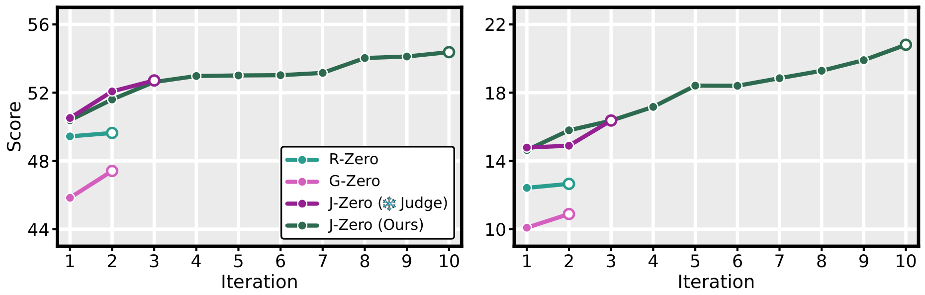
Self-play post-training with a frozen reward model imposes a hard ceiling: once the Solver saturates what the Judge can discriminate, further RL degrades performance. This is well-documented in verifiable-domain self-play systems (R-Zero, G-Zero), which typically peak within one to two iterations and then decline. In unverifiable domains — creative writing, open-ended instruction following — the problem is worse because the Judge is the only source of signal at all. J-Zero addresses both regimes by making the Judge itself a trainable participant in the self-play loop, supervised by preference pairs whose ordering is determined by construction rather than by the Judge’s own current scores.
Method
The system has three parameterized roles: Challenger C_{\theta_c}, Solver S_{\theta_s}, and Judge J_\phi. Each iteration runs three sequential phases (5 Challenger steps, 15 Solver steps, 8 Judge steps in the reported setup).
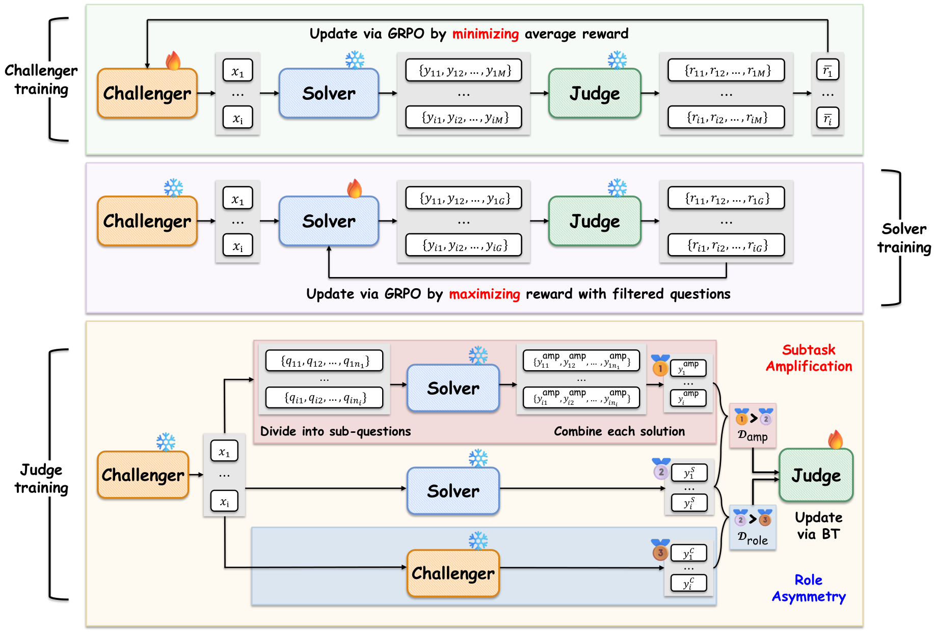
Adversarial Challenger–Solver game (Judge frozen). For each generated task x_i \sim C_{\theta_c}, the Solver samples M responses y_{i,j} \sim S_{\theta_s}(\cdot \mid x_i), scored by
r^{S}_{i,j} = \sigma\!\left(J_\phi(x_i, y_{i,j})\right) \in [0,1].
Solver and Challenger optimize
\min_{\theta_c}\mathcal{L}_C(\theta_c;\theta_s,\phi),\qquad \max_{\theta_s}\mathcal{R}_S(\theta_s;\theta_c,\phi),
with \mathcal{R}_S = \mathbb{E}_{x\sim C,\, y\sim S}[\sigma(J_\phi(x,y))] and \mathcal{L}_C = -\mathbb{E}[r_i^C], where r_i^C combines the negated Solver reward with auxiliary penalties for repetition and malformed tasks (making the game adversarial but not strictly zero-sum).
Judge update (Challenger and Solver frozen). This is the key contribution. The Judge is trained with a standard Bradley–Terry loss on two in-loop preference datasets whose orderings are known a priori:
- \mathcal{D}_{\text{role}} (role asymmetry): for a task x produced by the Challenger, the Solver’s response is labeled preferred over the Challenger’s own response to x. The prior is that a policy specialized to answering will outproduce a policy specialized to asking.
- \mathcal{D}_{\text{amp}} (subtask amplification): the Solver’s decompose-and-recombine answer is labeled preferred over its one-shot answer. This provides supervision above the Solver’s single-pass frontier — a form of process-level self-distillation.
Crucially, neither label set uses the current Judge scores, so the Judge cannot collapse into a fixed point of its own preferences.
Reliability of the constructed labels
The authors validate labels with an external LLM judge (Claude Opus 4.8), presented in both orders with ties dropped. Role-asymmetry labels agree with the external judge from 87.9\% at iteration 1, decaying to \approx 66\% as the adversarial curriculum drives tasks toward the Solver’s capability frontier and the quality gap between Solver and Challenger narrows. Subtask-amplification labels start unreliable — 21.1\% at iteration 1, because decomposition helps only when subtasks are individually solvable — cross 50\% at iteration 4, and reach 70\text{–}80\% later. The two curves crossing mid-training is what keeps the Judge supervised throughout: role asymmetry carries the early phase, amplification the late phase.
Results
On Qwen3-4B-Base and Qwen3-8B-Base, evaluated across 11 verifiable benchmarks (7 math, 3 general reasoning, IFEval) and 3 unverifiable ones (AlpacaEval 2.0, Arena-Hard-v2.0, EQ-Bench Creative Writing v3), against R-Zero and G-Zero baselines using Skywork-Reward-V2-Llama-3.1-8B as the initial Judge:
- Average improvement of +4.2 points on verifiable tasks and +8.0 on unverifiable tasks over the baselines.
- The larger gain in unverifiable domains is consistent with the hypothesis that a fixed reward model bottlenecks self-play most severely where verification is otherwise absent.
The continuity plot makes the ceiling argument concrete: baselines plateau or degrade after ~2 iterations, while J-Zero continues improving through at least 10.
The paper also reports that Judge co-evolution improves RM-Bench score, an independent reward-model benchmark disjoint from the in-loop preference construction — evidence that the co-adaptation is not merely fitting the Solver’s idiosyncrasies.
Limitations and open questions
- Scale is bounded at 8B for all three roles, and only base (non-reasoning) models are used; behavior with long-CoT reasoners is untested.
- The Judge is a discriminative BT classifier initialized from an off-the-shelf reward model, while Challenger/Solver share a generative init. Unifying all three roles under a single generative backbone (LLM-as-a-judge with critiques as richer supervision) is the natural next step but requires figuring out how to co-adapt a generative Judge without label collapse.
- The role-asymmetry label reliability decays over training; whether this eventually breaks the Judge at longer horizons than 10 iterations is unclear.
- The composite Challenger reward r_i^C hides several auxiliary terms whose weighting likely matters for stability but is not analyzed in the main text.
Why this matters
The result reframes zero-data self-play: the binding constraint is not policy capacity or task generation, but evaluator ceiling. J-Zero shows that a Judge can be trained inside the loop using construction-based preference orderings — cheaper than human labels, and, unlike Judge-score-derived labels, non-circular — enough to extend useful self-improvement from ~2 to ~10 iterations, particularly in unverifiable domains where no external verifier exists.
Source: https://arxiv.org/abs/2608.26582
Rubric-to-Code Credit Assignment for Reinforcement Learning
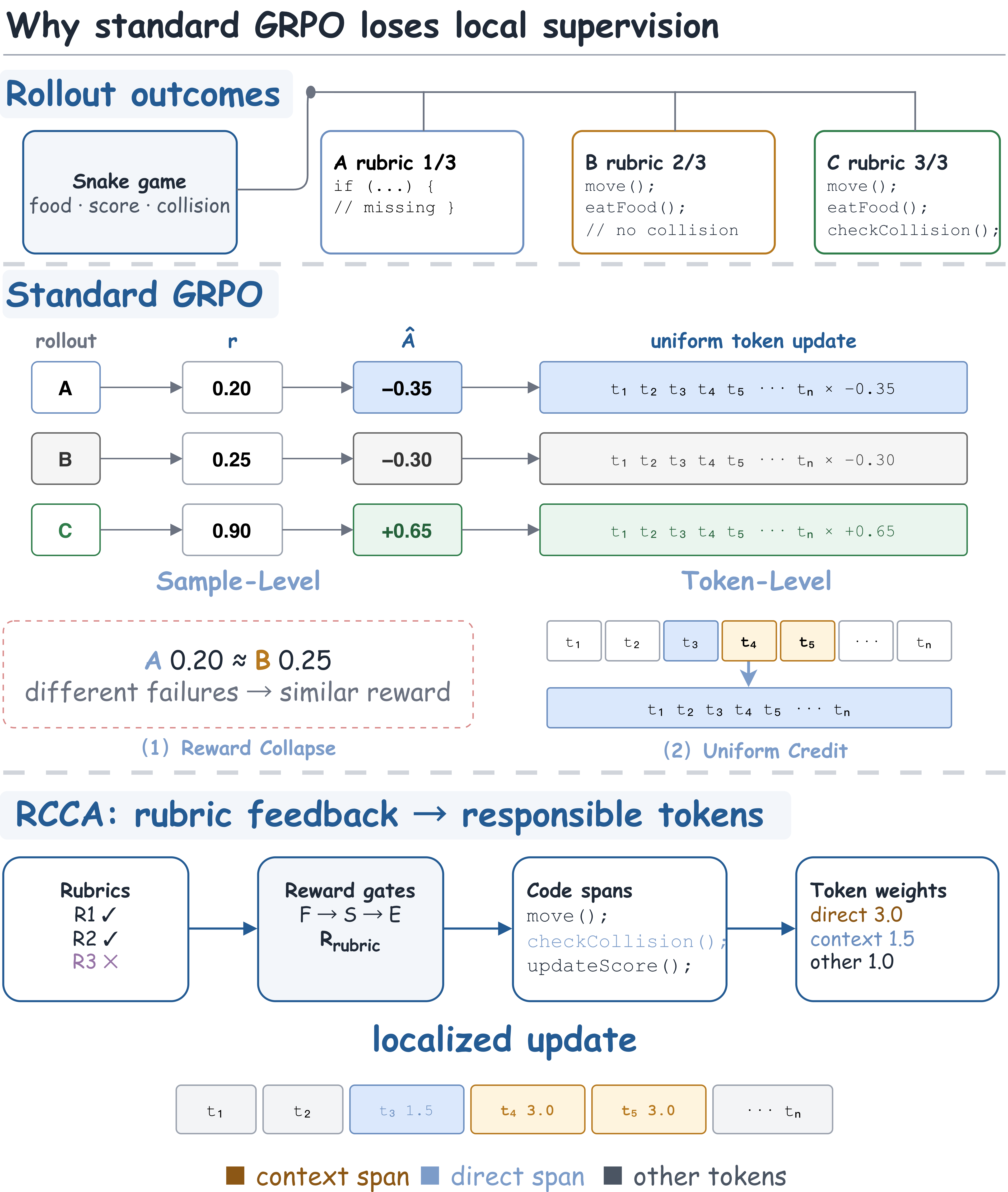
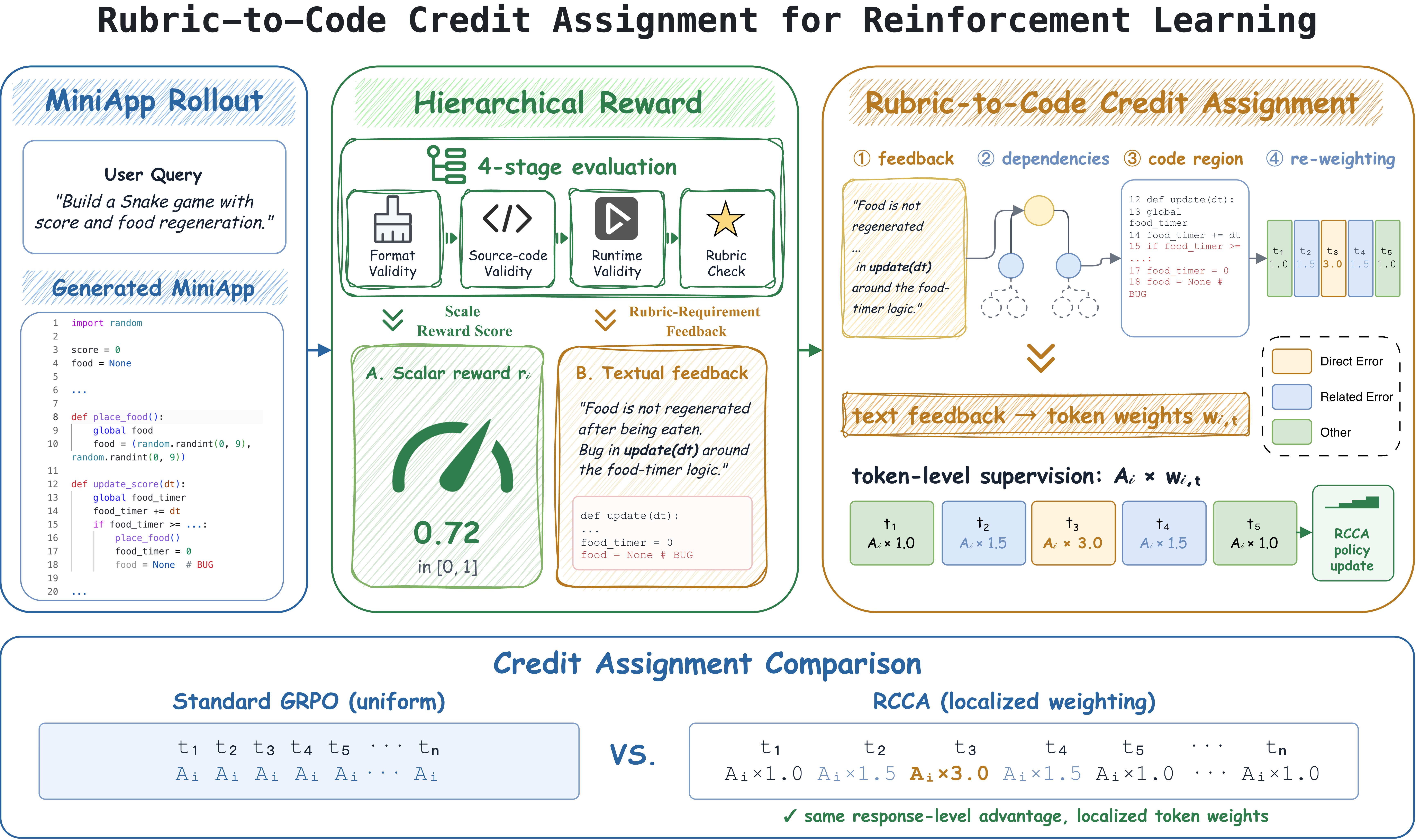
Interactive web application generation stresses RL fine-tuning in a way standard code benchmarks do not: a single natural language prompt yields an HTML/CSS/JS artifact whose quality decomposes into many largely independent user-facing behaviors — an initial rendered state, a click handler, a form validation rule, a CSS transition. Each behavior is realized in a localized code region (an event handler body, a DOM fragment, a specific selector). Standard GRPO collapses all of this into one scalar reward per rollout and multiplies the group-relative advantage across every generated token. Two failure modes follow: (i) rollouts with qualitatively different defects receive similar scalar rewards, flattening the intra-group advantage signal, and (ii) tokens irrelevant to the observed failure receive the same gradient weight as tokens in the offending region. RCCA (Rubric-to-Code Credit Assignment) attacks both.
Setup and hierarchical reward
Each task carries a rubric set \mathcal{R}=\{r_1,\dots,r_M\}, where each r_i specifies one user-facing requirement (an expected initial state, a triggered interaction outcome, a style constraint). Rubrics are the atomic unit of evaluation and of credit attribution.
To de-collapse the sample-level signal, RCCA scores rollouts under a hierarchy that separates failure classes rather than averaging them:
- output-format validity (is the response parseable as HTML/CSS/JS?),
- source-code validity (does it lint/parse?),
- runtime validity (does it execute without throwing in a headless browser?),
- rubric-level requirement satisfaction (fraction of r_i passed by an evaluator).
Because these tiers dominate lexicographically, rollouts with different failure modes end up at different points in reward space, restoring discrimination inside each GRPO group and thus non-degenerate group-relative advantages.
Localization and token-level credit
The token-level contribution is the more novel piece. For each detected rubric failure, an evaluator emits a textual diagnostic (which requirement failed, and why). RCCA aligns that diagnostic against the generated code to identify the responsible span — e.g., the specific event handler or CSS selector — and then maps those characters back to the token indices in the rollout. Tokens inside attributed spans receive amplified advantage; tokens outside receive the standard GRPO weight. Conceptually the objective becomes
\mathcal{L}_{\text{RCCA}} = -\mathbb{E}\!\left[\sum_{t} w_t\,\hat{A}_{\text{group}}\,\log \pi_\theta(y_t \mid y_{<t}, x)\right],
with w_t > 1 on tokens localized to the rubric-attributed span and w_t = 1 elsewhere, while \hat{A}_{\text{group}} is the group-relative advantage induced by the hierarchical reward. The advantage itself is now shaped by rubric-level pass rates rather than a single scalar, and its per-token application is masked by evaluator-derived attributions rather than uniform.
Training pipeline and results
The base is Ling-3.0-Flash, a 124B-parameter hybrid-linear MoE with 5.1B activated parameters per token. Training runs in two stages: SFT to bootstrap artifact-generation capability, then RCCA on top. Evaluation uses MiniAppBench (interactive web app generation, the primary benchmark) and ArtifactsBench (broader visual/interactive artifacts, for generalization).
On MiniAppBench, Ling-RCCA-Flash reaches 41.25, a +32.20 point gain over Ling-3.0-Flash, and slightly exceeds Claude Opus 4.5 on that benchmark. On ArtifactsBench, it reaches 76.19, indicating the localized credit signal does not overfit to the training-time rubric distribution but transfers to a benchmark that mixes visual and interactive criteria. The magnitude of the MiniAppBench delta is the more interesting number: closing a 32-point gap on top of an SFT’d base implies that the dominant source of remaining error was not capability but credit assignment — the base could produce most of the required code somewhere in its rollouts but GRPO could not reliably reinforce the correct fragments.
Limitations and open questions
- Attribution quality is bounded by the evaluator. If the diagnostic-to-code alignment picks the wrong span (a common failure when a bug spans multiple regions, e.g., a state variable declared far from where it is misused), the token-level weight amplifies the wrong gradient. The paper does not report robustness of the aligner in isolation.
- The hierarchical reward is lexicographic in construction; there is no ablation reported here on whether the sample-level gain comes primarily from the tier separation or from the rubric pass-rate signal within tier 4.
- Rubrics must exist. Extending RCCA to domains where user-facing requirements are not enumerable (open-ended design tasks, long-form reasoning) is unclear.
- Contamination and evaluator-model coupling between MiniAppBench training rubrics and evaluation are not discussed in the excerpt.
Why this matters
RCCA is a concrete instance of turning structured, verifier-decomposable rewards into spatially localized RL signals, rather than throwing them away at the reward-aggregation step. For any domain where an artifact’s quality is a conjunction of locally-realized requirements — UI generation, multi-file code edits, tool-augmented agents — this is a more faithful credit-assignment recipe than sequence-level GRPO, and the 32-point MiniAppBench jump suggests the loss from uniform advantage weighting has been substantially underestimated.
Source: https://arxiv.org/abs/2608.27906
LoopArena: Benchmarking Models as Runtime Controllers for Loop Engineering
Problem
“Loop Engineering” refers to the practice of wrapping a coding agent in an outer loop that monitors progress, dispatches subtasks, runs verification, and decides when to stop. In deployed agent systems, this outer controller is increasingly a separate model call from the coding worker. Standard coding-agent benchmarks (SWE-Bench-style) score the end-to-end stack, conflating the worker’s coding ability with the controller’s guidance quality. If a run fails, it is not attributable: the controller may have trusted a stale progress note, skipped verification, or stopped prematurely — or the worker may simply have been unable to execute a correct plan.
LoopArena isolates the controller. The worker is held fixed (Qwen3.7-Plus in all reported runs), and the model under evaluation only issues structured “Loop Contracts” that direct the worker’s next round.
Harness and roles
Three model roles are pinned by the harness (Figure 1):
- Worker: the only role with repository and tool access; edits code and runs commands.
- Reporter: a temporary agent instantiated from the same model configuration as the worker; has read-only workspace access and produces four required fields —
task_context_and_constraints,work_history_and_current_state,verification_and_evidence,open_issues_and_uncertainty— with citations to specific worker turns. Not appended to the persistent worker conversation. - Controller: receives the deterministically rendered Evidence Packet plus cited worker turns and the turn-budget state. It returns a structured decision with
action ∈ {advance, verify, stop}and, for non-stop actions, aworker_instruction(goal, context, required_outcomes, prohibited_actions, completion_condition),protected_invariants, and averification_acceptance_condition.
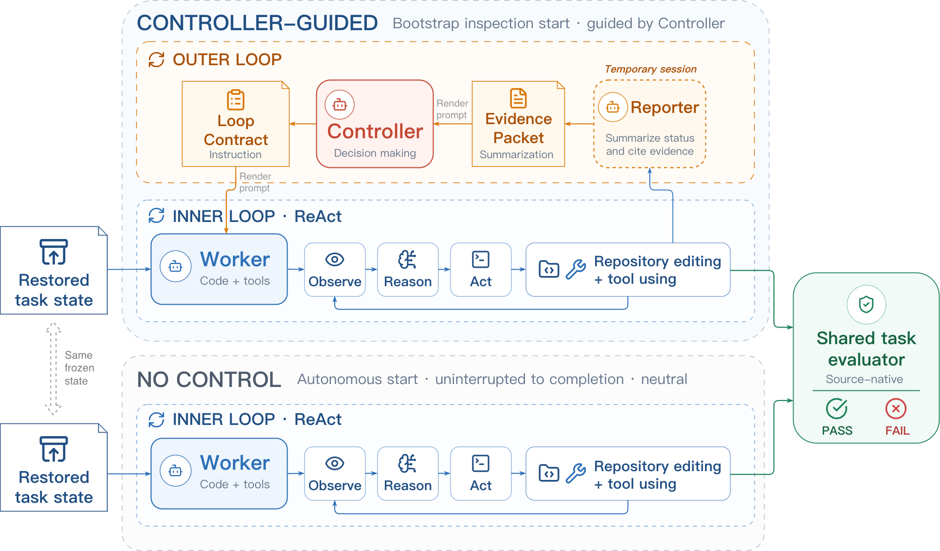
The controller has no tools and never edits the repository directly; its output is the Loop Contract that the harness renders as the worker’s next user turn.
Three evaluation types
The benchmark spans a cost/scope axis (Figure 2):
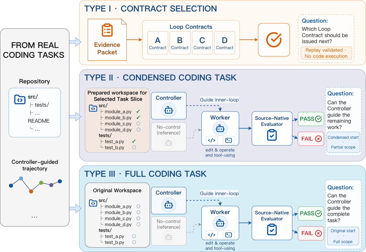
Type I — Contract selection: single frozen control point, four candidate contracts, no worker execution at eval time. Correct-option construction is nontrivial. For each item, one recorded contract plus three plausible alternatives (authored under a balanced model-family assignment) are replayed from the restored state under two seed schedules S+10^6 and S+2\cdot10^6, holding worker, budget, evaluator, continuation policy, and stopping rules constant. Terminal task success is primary; ties broken by fewer controller cycles, then fewer worker turns. An item is retained only if both schedules identify the same unique winner. Metric: \operatorname{Acc}_{\mathrm{I}}(\pi) = \frac{1}{N_I}\sum_{q=1}^{N_I} \mathbf{1}[\widehat{j}_{\pi,q}=j_q^\star].
Type II: repeated control over a prepared task-slice starting workspace, with real worker execution.
Type III: repeated control from the original task state through completion.
Source tasks come from SCBench (long-horizon iterative coding) and BeyondSWE (multi-stage SWE). The benchmark has 90 Type I questions and 27 paired Type II/III instances (11 SCBench + 16 BeyondSWE).
Type I results
Five controllers were evaluated: Qwen3.7-Plus, DeepSeek-V4-Flash-0731, GLM 5.2, GPT-5.5, and Claude Opus 4.8. All controllers produced valid parses on 100% of items (Invalid Rate = 0.00%).
| Controller | Correct/90 | Acc (%) | Cost ($/90) |
|---|---|---|---|
| Qwen3.7-Plus | 65 | 72.22 | 0.70 |
| DeepSeek-V4-Flash-0731 | 70 | 77.78 | 0.31 |
| GLM 5.2 | 67 | 74.44 | 3.02 |
| GPT-5.5 | 79 | 87.78 | 9.43 |
| Claude Opus 4.8 | 69 | 76.67 | 13.68 |
GPT-5.5 leads by 10 points over the next controller. The cost spread across controllers is roughly 44×, and DeepSeek achieves the second-best accuracy at the lowest cost, indicating that raw model scale is not the sole determinant of contract-selection quality. The source-decomposed table shows GPT-5.5 dominates on both subsets (87.50% SCBench, 88.00% BeyondSWE), while Claude Opus 4.8 shows a notable gap between SCBench (82.50%) and BeyondSWE (72.00%). Since the SCBench/BeyondSWE subsets differ in both tasks and item counts (40 vs. 50), the paper explicitly declines to use these splits for ranking.
Method notes worth flagging
The construction protocol has two properties that matter for interpreting results. First, the recorded contract from the source trajectory is not privileged: the confirmed winner is whichever candidate wins under both replay schedules, so items where the “human/agent picked” option was suboptimal are retained honestly. Second, rejection is aggressive — items with no unique winner, or where the two schedules disagree, are dropped rather than repaired. This trades benchmark size for answer-key validity.
The comparison table (Table 16) draws a clean distinction from adjacent paradigms: final-state coding benchmarks evaluate the coding stack; interactive-agent benchmarks evaluate the agent-plus-scaffold; loop-system benchmarks evaluate the entire submitted loop system including its coding model. LoopArena is the only setting that pins the coding model and evaluates only the loop-control decisions.
Limitations and open questions
- Type II/III results are not present in the provided sections, so the central claim — whether Type I accuracy ranks controllers consistently with executable settings — is not yet verifiable here. The paper’s stated goal of using Type II as a cheaper proxy for Type III depends on rank correlation between them.
- All executable evaluation uses a single worker (Qwen3.7-Plus). Controllers may generalize differently over worker capability; a controller tuned to compensate for a weak worker may look worse when paired with a strong one.
- 90 Type I questions and 27 paired tasks is small; per-controller differences of a few items shift accuracy by 1–2 points.
- The Reporter uses the same configuration as the worker. If the Reporter systematically mischaracterizes state, all controllers inherit that bias, and the benchmark measures decision quality conditional on that reporter’s evidence, not on ground truth.
- Contract selection is a 4-way multiple choice; the executable settings measure open-ended contract generation. These are related but not identical skills.
Why this matters
Loop Engineering is becoming the dominant deployment pattern for coding agents, yet the community has no principled way to attribute end-to-end success to the outer controller vs. the inner worker. LoopArena’s tiered design — with an execution-free Type I whose answer keys are validated by replay under matched seed schedules — offers a reproducible way to score controller models directly, which is prerequisite for iterating on prompt scaffolds, controller fine-tuning, or specialized “planner” models.
Source: https://arxiv.org/abs/2608.28281
Agentic Artifact Creation: Systems, Evaluation, Principles, and Opportunities
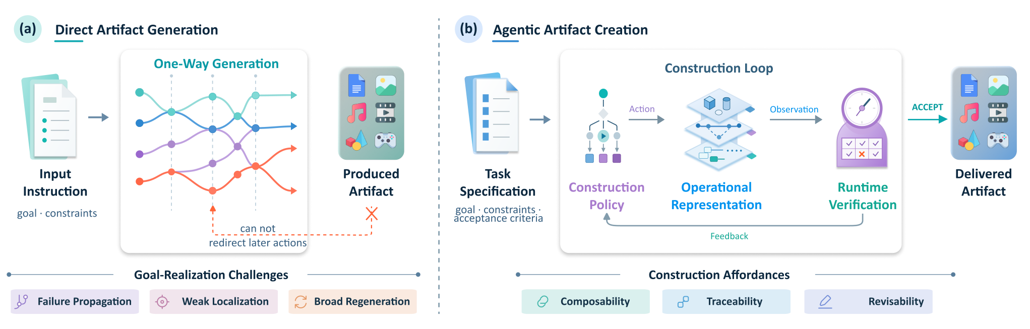
This survey covers 259 works through August 20, 2026 (230 systems, 29 benchmarks) and proposes a functional definition of “agentic artifact creation” that separates it from single-pass generation and from generic agent frameworks. The unit of analysis is a single artifact-creation episode: it qualifies as agentic when an AI system (i) materially constructs or revises the delivered artifact, (ii) carries artifact or process state across construction decisions, and (iii) uses at least one intermediate observation to redirect later work — the next action, the revision target, the active branch, or the stopping decision.
The paradigm and its functional decomposition
The screening rule is stateful construction with redirection. Direct pipelines with post-hoc filtering fail the definition because observations do not steer subsequent artifact-side actions; iterative and mixed-initiative systems pass when the three conditions hold. Architecturally, the authors factor every such episode into three roles: an Operational Representation (an intermediate form plus an edit interface that exposes addressable state), a Construction Policy (decision control and agent topology), and Runtime Verification (an observation source and a feedback function that returns status, diagnosis, or guidance).
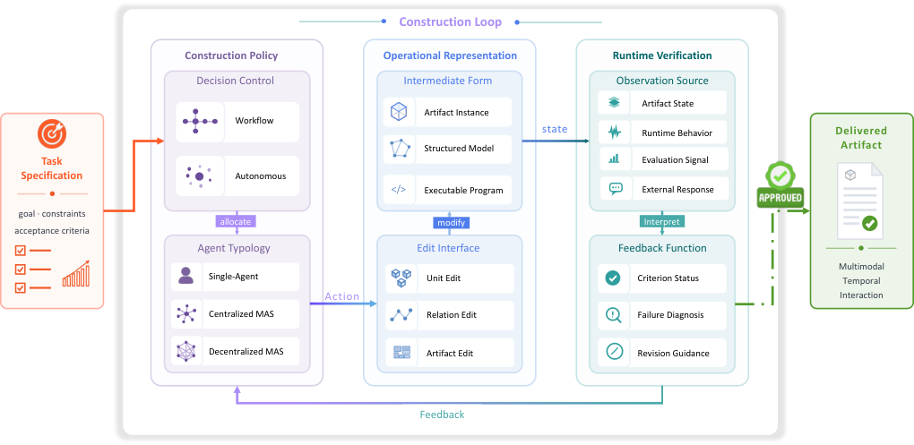
This decomposition is used consistently in the system tables. For example, STORM is coded as \text{Outline} \xrightarrow{\text{Agents}} \text{Article} with a unit-plus-relation edit interface and a centralized MAS topology; AI Scientist as \text{Manuscript} \xrightarrow{\text{LaTeX}} \text{Paper} with runtime-plus-metric verification producing status, diagnosis, and guidance; MCQG-SRefine uses draft-critique loops with state and metric signals feeding the same three-part diagnosis. The taxonomy is deliberately behavioral, not architectural: multi-agent orchestration is neither necessary nor sufficient.
Six artifact families and observability
The literature is partitioned by the primary independently accepted artifact form: textual, 2D visual, audio, video, spatial, and behavioral. Family assignment follows which failure would render the deliverable unacceptable and what state is needed to repair it. Table 2 in the paper maps each family to dependency regimes (semantic, perceptual, spatial, temporal, dynamic) and observation modes (reading, rendering, playback, interaction). The salient pattern: textual and 2D-visual artifacts fail under static inspection; audio and video fail during temporal playback; spatial and behavioral artifacts fail only under traversal, execution, or interaction — so failure observability is delayed, and repairability depends on whether local edits preserve upstream commitments.
This produces the paper’s core qualitative lens along three axes: decision interdependence (how much one decision constrains other state), failure observability (whether failures become visible and attributable in time), and repairability (whether a diagnosis maps to a bounded action that preserves accepted work). Narrative, long-form video, and world-construction systems are cited as canonical cases of delayed or incomplete observability; repository-scale code benchmarks illustrate long-range dependency failure modes where locally plausible edits break cross-module contracts.
Applications and evaluation
Applications are treated as an orthogonal dimension: creative production, brand communication, educational support, professional work, scientific research, and engineering design. The same artifact family serves different domains with different loci of acceptance — creator/audience experience, brand commitments, learning outcomes, professional judgment, scientific evidence, or executable/physical validity — and one workflow can require multiple families (e.g., interactive entertainment combines behavioral runtime validity with narrative and stylistic coherence).
The evaluation chapter insists that a claim identify five elements: target, criterion, metric, signal, and protocol. Targets separate into the delivered artifact, the construction trajectory, and the agentic system itself; the authors are explicit that aggregating artifact- or trajectory-level scores over a task suite supports task-capability claims but not system-level claims (efficiency, robustness, controllability), which require repeated runs, controlled operating conditions, resource tradeoffs, or version contrasts. Evidence channels (compiler, renderer, simulator, specialist model, LM judge, human) and evaluator types are declared orthogonal — a compiler used inside a stated protocol is evaluation evidence; used inside a repair loop it is Runtime Verification.
Four principles and six open problems
The synthesis distills four principles around an addressable artifact state: (1) Externalize Commitments — encode requirements, source links, constraints, dependency edges, provenance, and review status as artifact-side state rather than policy-side memory (Crafter’s typed figure revisions and CADIR’s editable executable CAD graph are cited as exemplars); (2) Define Control Boundaries — assign decision responsibility along dependency and consequence gradients; (3) Make Feedback Actionable — bind evidence to bounded repair actions; (4) Revalidate Affected State — perform selective revalidation on change. The first is definitional, the middle two synthesize recurring design patterns, and the fourth is flagged as backed by comparatively sparse evidence.
Section 8 names six unresolved control problems: global coherence under decision interdependence, repair under diagnostic blind spots, durable system evolution, changing creator intent, authority under delegation, and evaluation when multiple outcomes are valid. A concrete research direction proposed is automated representation search: a typed commitment graph linking requirements to artifact units, decisions, owners, and evidence, materialized only for links touched by a change or judged high-risk, with held-out changes testing whether a lighter representation preserves coherence without excessive rework, stale evidence, or coordination overhead.
Limitations
The taxonomy is behavioral and often coarse — many systems are coded with “NR” (not reported) for observation source and feedback function, reflecting under-reporting in the literature rather than the survey’s design. Comparative quantitative claims across families are avoided; the difficulty lens is qualitative and explicitly not a maturity ladder. The revalidation principle is acknowledged as thinly evidenced.
Why this matters
The survey provides a testable definition and a common vocabulary (Operational Representation, Construction Policy, Runtime Verification) that lets readers compare, e.g., a poster-generation MAS and a repository-level coding agent on the same axes of interdependence, observability, and repairability, and forces evaluation claims to declare target, criterion, metric, signal, and protocol — a discipline currently missing from most agentic-system papers.
Source: https://arxiv.org/abs/2608.28122
Hacker News Signals
How to build a diffusion language model
Source: https://kuleshov-group.github.io/blog/blog/2026/how-to-build-a-diffusion-language-model/
A practical walkthrough of masked diffusion language models (MDLMs), covering the full training and inference pipeline at enough depth to be useful as an implementation guide. The core idea: instead of autoregressive next-token prediction, a forward process gradually masks tokens according to a noise schedule, and the model learns to denoise — predicting masked tokens given the partially observed sequence.
The forward process absorbs tokens into a mask state [M] with rate \beta(t), so at time t each token is independently masked with probability \alpha(t). The reverse process learns p_\theta(x_0 | x_t) directly — not a one-step denoiser, but a clean-sequence predictor that parameterizes the reverse marginal. The training objective reduces to a weighted cross-entropy over masked positions:
\mathcal{L} = \mathbb{E}_{t, x_0, x_t}\left[\frac{\beta(t)}{1 - \alpha(t)} \sum_{i: x_t^i = [M]} \log p_\theta(x_0^i | x_t)\right]
Inference uses a discretized reverse chain: at each step, re-mask a fraction of currently unmasked tokens and re-predict from the full noisy context, which allows arbitrary-order generation unlike autoregressive models. The post covers practical choices — absorbing vs. uniform noise, the effect of the noise schedule shape, how to handle semi-autoregressive chunked decoding to trade quality for speed, and classifier-free guidance adapted for discrete diffusion.
Key engineering notes: the model architecture is essentially a standard bidirectional transformer with no causal mask, which gives full context over the partially masked sequence. The bidirectionality is the structural win over AR models — every position attends to every other unmasked position, potentially improving coherence on long-range dependencies.
The post is honest about where MDLMs still lag: perplexity on standard benchmarks remains worse than comparably sized AR models, and sampling latency is not obviously better unless you use aggressive parallelism. Open questions include better noise schedules, improved guidance mechanisms, and whether the bidirectional context advantage actually materializes on downstream tasks.
Why this matters
MDLMs represent the most credible non-autoregressive architecture for language so far; a clean implementation guide lowers the barrier for empirical comparison against AR baselines.
Continuous Diffusion Language Models (CDLMs)
Source: https://sander.ai/2026/08/24/continuous-dlms.html
Sander Dieleman’s post addresses a fundamental tension: diffusion is native to continuous spaces, but language is discrete. The standard fix — embedding tokens and adding Gaussian noise in embedding space — breaks down because the geometry of embedding space is not semantically uniform, so noising toward zero or a Gaussian prior does not correspond to meaningful interpolation between tokens.
The post proposes and analyzes CDLMs, which operate diffusion entirely in a learned continuous latent space rather than in raw token-embedding space. A separate encoder maps token sequences to continuous representations; the diffusion process runs on these representations with standard Gaussian forward noise q(z_t | z_0) = \mathcal{N}(z_t; \sqrt{\bar\alpha_t} z_0, (1-\bar\alpha_t)I); a decoder reconstructs token distributions from denoised latents. The key insight is that the encoder should be trained jointly so that the latent geometry is actually smooth with respect to semantic similarity — making the continuous diffusion assumption locally valid.
Dieleman distinguishes this from earlier approaches like Diffusion-LM, which worked directly in embedding space and required projection steps to stay near valid embeddings. CDLMs instead commit to continuous latents and use a soft reconstruction loss (cross-entropy against softmax decoder outputs) rather than hard projection, which keeps gradients well-behaved throughout.
The post covers practical tradeoffs: latent dimensionality (too low loses information, too high makes denoising harder), the role of the KL term if a VAE-style bottleneck is used, and how classifier-free guidance translates — conditioning information is injected into the denoising network, with the decoder remaining unconditional. Inference requires running the full reverse diffusion chain then decoding, which is slower than AR generation but fully parallelizable across sequence positions.
Limitations acknowledged: training instability when encoder, diffusion model, and decoder are optimized together; sensitivity to the choice of noise schedule relative to the scale of the latent space; and the lack of a clean likelihood lower bound comparable to the ELBO in VAE-based models.
Why this matters
A principled continuous-space treatment of language diffusion is necessary for scaling these models; this post clarifies the geometric requirements that prior discrete-noise and embedding-space approaches quietly violated.
RISC-V is now officially supported by CPython
Source: https://blog.python.org/2026/08/riscv-now-officially-supported/
CPython has promoted RISC-V (specifically RV64GC, the standard 64-bit general-purpose profile with compressed instructions) to a Tier 1 supported platform, meaning it now has the same CI coverage and release guarantees as x86-64 and aarch64. This is not a trivial status change: Tier 1 requires that the buildbot infrastructure continuously runs the full test suite, that release binaries are published, and that regressions on that platform block releases.
The technical work involved several layers. CPython’s JIT compiler (introduced in 3.13 as a copy-and-patch JIT) needed RISC-V code generation templates; the calling convention follows the RISC-V psABI with integer arguments in a0-a7 and floating-point in fa0-fa7, and the JIT templates had to correctly handle the two-instruction sequence required for PC-relative addressing beyond ±2GB (AUIPC + ADDI/JALR pairs, since RISC-V lacks a single large-immediate load). The GC’s stack scanning also required RISC-V-specific unwind information.
Beyond the JIT, the ctypes and cffi-compatible FFI layer needed the RISC-V ABI’s struct-passing rules, which differ from x86-64: small structs are passed in register pairs rather than as single integer-width values when they contain mixed int/float fields, following hardfloat ABI rules.
The practical motivation is clear: RISC-V is increasingly deployed in embedded and edge hardware, single-board computers, and as the baseline ISA for custom AI accelerators where Python tooling for model deployment is expected. Having CPython as Tier 1 means NumPy, PyTorch (to the extent it avoids ISA-specific intrinsics), and the broader ecosystem can reliably target these platforms without per-vendor patches.
The remaining gap is RISC-V vector extension (RVV) support in the numerical stack — NumPy and SciPy still rely on explicit SIMD backends, and RVV’s variable-length vector model requires different intrinsic handling than fixed-width SSE/AVX or NEON.
Why this matters
Tier 1 status removes Python as a portability bottleneck for RISC-V deployment, which matters most for the embedded ML inference and edge compute use cases driving RISC-V adoption.
HTTPX2 – A next-generation HTTP client for Python
Source: https://github.com/pydantic/httpx2
Pydantic’s HTTPX2 is a ground-up rewrite of the HTTPX HTTP client, retaining the familiar sync/async dual API while addressing architectural complaints that accumulated in the original. The headline changes are: HTTP/3 (QUIC) support as a first-class transport, a revised connection pool with per-host and global concurrency limits enforced without the lock contention issues in HTTPX’s original pool, and a type-safe request/response model that integrates with Pydantic v2 validation directly.
The transport layer is structured as a clean protocol stack: AsyncTransport is the base interface, with HTTP/1.1, HTTP/2 (via h2), and HTTP/3 (via aioquic) as pluggable implementations selected by ALPN negotiation or explicit configuration. This lets users swap in mock transports for testing without monkey-patching, a longstanding pain point.
Connection pooling now tracks connections by (scheme, host, port) key with configurable max_connections and max_keepalive_connections, and uses an async semaphore per key rather than a global lock, reducing head-of-line blocking under concurrent requests to multiple hosts. The original HTTPX used a single threading.Semaphore in sync mode and an asyncio.Semaphore in async mode but shared internal state in ways that caused subtle races under high concurrency.
The request model wraps body content as typed streams — ByteStream, AsyncByteStream, MultipartStream — with explicit backpressure, which matters for large uploads where the original would buffer aggressively. Response bodies similarly expose aiter_bytes() and aiter_lines() as async generators.
Pydantic integration means response JSON can be parsed directly into model types via response.parse(MyModel), with validation errors surfaced as ResponseValidationError rather than raw ValidationError, giving cleaner error messages in API client code.
Limitation: HTTP/3 support depends on aioquic, which has its own OpenSSL/BoringSSL dependency chain that complicates packaging, particularly on platforms where system OpenSSL is old. The library is also new enough that edge cases in QUIC connection migration and 0-RTT resumption are likely not fully tested.
Why this matters
A properly layered, type-safe HTTP client with HTTP/3 fills a real gap in the Python ecosystem, particularly for async service clients where HTTPX’s original pool behavior caused production issues.
Building my own network stack
Source: https://blog.lyc8503.net/en/post/dn42-2-dnet/
A detailed writeup on implementing a userspace network stack in the context of DN42, the hobbyist overlay network that uses real BGP, real address space allocation, and real routing protocols to simulate an internet-scale AS topology. The author builds dnet, a userspace TCP/IP stack that bypasses the kernel network stack entirely using TUN/TAP interfaces.
The implementation follows the standard layered model but with enough specifics to be instructive. At the IP layer, the author implements fragmentation and reassembly with a reassembly buffer keyed by (src, dst, protocol, id) and a timeout to garbage-collect incomplete fragments — a detail often glossed over. ICMP is handled for both error reporting and echo, with the ICMP checksum computed over the ICMP header and payload only (not a pseudo-header, unlike TCP/UDP).
The TCP implementation covers the core state machine (SYN/SYN-ACK/ACK, FIN/FIN-ACK, RST handling) plus the send and receive buffers as ring buffers with sequence-number arithmetic. The author handles the tricky cases: simultaneous open, TIME_WAIT and its 2MSL timer, and TCP keepalives. Congestion control is simplified to a basic slow-start with a fixed ssthresh, acknowledging that real congestion avoidance (CUBIC, BBR) would require significantly more state.
The TUN interface integration is straightforward: open /dev/net/tun, set IFF_TUN | IFF_NO_PI flags, assign an IP address, and read/write raw IP packets. The author uses Rust with tokio for the async I/O loop, with each connection mapped to a task.
DN42 integration means the stack also handles BGP session establishment (using an external BGP daemon, Bird2, rather than implementing BGP from scratch) and correct handling of the DN42 address ranges (172.20.0.0/14, fd00::/8 for IPv6).
Known limitations: no IP options handling, no TCP urgent data, and the congestion control is too simple for real-world use. The implementation is explicitly educational rather than production-ready.
Why this matters
Working through a real protocol stack against a live BGP network exposes corner cases that simulators hide; the writeup is a useful reference for anyone implementing network protocols from scratch.
Benchmarking Pocket-Scale Inference
Source: https://artificialanalysis.ai/hardware-inference-stack/mobile-phones
Artificial Analysis benchmarks LLM inference performance on consumer mobile hardware — primarily flagship Android SoCs (Snapdragon 8 Elite, Dimensity 9400) and Apple Silicon (A18 Pro, M-series in iPad/MacBook) — using a consistent methodology across on-device inference frameworks including llama.cpp, MLC-LLM, and platform-native options like Apple’s Core ML and Google’s MediaPipe LLM.
The core metrics are tokens per second for prefill and decode phases separately, memory bandwidth utilization (inferred from model size and observed throughput), and model quality on standard benchmarks at the quantization levels that actually fit in device RAM. Most tested models are 1B-8B parameter range at 4-bit or mixed 2/4-bit quantization; the 8B models only fit comfortably on devices with 12GB+ RAM.
Key findings from the numbers: Apple’s Neural Engine delivers high throughput on quantized weights for models optimized via Core ML (ANE), but the ANE’s limited SRAM means long-context prefill degrades significantly compared to GPU-side execution. Snapdragon 8 Elite’s Hexagon NPU shows competitive decode throughput on llama.cpp with its QNN backend, often outperforming the GPU path for small batch sizes due to lower memory bandwidth pressure. The Dimensity 9400’s APU shows strong performance-per-watt but requires vendor-specific SDK integration that most open frameworks don’t fully exploit.
The methodology note: all benchmarks run at thermal steady state after a warm-up period, not peak burst performance, which is a meaningful difference on mobile where sustained throughput drops 30-50% from cold-start peaks due to thermal throttling.
Gaps identified: no multi-modal benchmarking (vision encoders on mobile NPUs), no measurement of prompt caching effectiveness on devices with persistent KV cache support, and the lack of standardized battery drain metrics makes energy efficiency comparison indirect.
Why this matters
On-device inference avoids latency and privacy costs of cloud inference; these numbers clarify which hardware generations and frameworks are actually viable for sub-second response workloads.
Tether: iMessage, SMS, etc. on Linux
Source: https://zackbartel.com/blog/2026/08/tether/
Tether is a tool that proxies iMessage, SMS, and other Apple-ecosystem messaging through a paired iPhone to a Linux desktop, without requiring a Mac in the loop. This is technically interesting because there is no official API — the approach reverse-engineers the communication channel between Macs and iPhones used by Continuity features.
The architecture has two components: a small agent running on the iPhone (requiring a jailbreak or developer-mode sideloading depending on iOS version) that intercepts and forwards messages, and a Linux daemon that communicates with the agent over a local network or USB tunnel. USB tunneling uses usbmuxd, the same daemon that iTunes and libimobiledevice use to multiplex TCP connections over the iPhone’s USB interface, so no network configuration is needed when the phone is physically connected.
On the iPhone side, the agent hooks into MessagesKit.framework or the lower-level IMCore private framework to receive and send messages without going through the Messages app UI. The exact hooking mechanism depends on iOS version — on jailbroken devices it uses a dyld interpose or Cydia Substrate tweak; on non-jailbroken devices with developer mode, it uses an XPC service approach that has more limited access.
The Linux daemon exposes a local socket with a simple JSON protocol, and a reference client implements a terminal UI using notcurses. The protocol covers send, receive, read receipts, and reactions, but not FaceTime, SharePlay, or file transfers beyond images (which are base64-encoded inline).
The critical limitation is Apple ID authentication: iMessage uses end-to-end encryption via the IDS (Identity Directory Service) protocol, and the agent on the phone handles all cryptographic operations using the phone’s existing credentials. This means Tether does not need to re-implement IDS key management, but it also means the Linux client has no independent iMessage identity — everything is proxied through the phone’s session.
Why this matters
For Linux users who need iMessage for professional communication, this is currently the only viable approach that doesn’t require keeping a Mac running; the technical approach of proxying through usbmuxd is reusable for other Continuity-feature bridging.
SQLite as a Document Database (2020)
Source: https://dgl.cx/2020/06/sqlite-json-support
This 2020 post resurfaces regularly because its core content remains accurate and underused. SQLite has shipped JSON support since 3.9.0 (2015) via the json_each() and json_extract() table-valued functions and the -> / ->> operators (added in 3.38.0, 2022). The post demonstrates using these to treat SQLite as a document store without sacrificing relational joins or ACID guarantees.
The key primitives: json_extract(data, '$.field') extracts a scalar from a JSON blob stored in a TEXT column; json_each(data, '$.array') expands a JSON array into rows with key, value, type, atom, id, parent, fullkey, and path columns, enabling joins against array elements. These compose with standard SQL aggregates and window functions without restriction.
The indexing story is important and often missed: SQLite supports expression indexes, so CREATE INDEX idx ON t(json_extract(data, '$.field')) creates a B-tree index on an extracted JSON field, giving point-lookup performance comparable to a dedicated column. Range queries and covering indexes work the same way. This eliminates the main performance objection to storing structured data as JSON.
The generated columns feature (3.31.0, 2020) improves on this further: ALTER TABLE t ADD COLUMN field TEXT GENERATED ALWAYS AS (json_extract(data, '$.field')) STORED materializes extracted values as a real column, making them queryable without the function call overhead and compatible with standard index syntax.
What this combination enables: schema-flexible storage (add fields to the JSON without migrations) with selective indexing on fields that appear in queries, relational joins across documents via standard FK columns alongside the JSON blob, and full ACID transactions — a superset of what most dedicated document databases offer for single-node workloads.
Limitations: JSON functions add parsing overhead on every access if extracted values are not indexed or materialized; no native JSON schema validation; and the query planner cannot use JSON-extracted values in multi-column indexes as effectively as native column types.
Why this matters
Most use cases that reach for MongoDB or DynamoDB for “flexibility” can be served by SQLite’s JSON support with better consistency guarantees and zero operational overhead, a point worth re-making as new developers encounter it.
Noteworthy New Repositories
kulkarnirohit123/cra-agent
An autonomous compliance agent targeting the EU Cyber Resilience Act. The pipeline chains repository scanning, vulnerability triage, issue tracking, and automated remediation: it scans source trees for CVEs and misconfigurations, classifies findings by CRA severity categories, opens Jira tickets with structured metadata, then generates pull requests containing patches. The agentic loop is built on top of a tool-using LLM backbone, with each stage (scan, triage, PR generation) implemented as a discrete tool call, allowing the orchestrator to retry or escalate. The practical value is reducing the manual compliance gap that teams face ahead of CRA enforcement deadlines — particularly for smaller engineering organizations without dedicated security staff. Configurable thresholds let teams tune what gets auto-fixed versus flagged for human review. The architecture is reasonably auditable because each agent action is logged before execution, giving a traceable decision trail regulators may want.
Source: https://github.com/kulkarnirohit123/cra-agent
PatilShreyas/debroid
A headless Android debugger exposing a programmatic interface intended for AI coding agents rather than humans. Debroid connects to a live Android process via ADB and the JDWP protocol, allowing an agent to inspect heap state, set and clear breakpoints, step through execution, and read local variables — all without a GUI IDE. The API surface is designed to be consumed by LLM tool calls: structured JSON in, structured JSON out. This matters because existing Android debugging is tightly coupled to Android Studio’s UI, making it opaque to autonomous agents. Debroid decouples the debugging capability from the IDE layer, enabling scenarios where an AI agent can iteratively probe a crashing app, collect runtime state, and correlate it with source changes. Useful for automated regression triage and for embedding debugging capability inside larger mobile-development agent pipelines.
Source: https://github.com/PatilShreyas/debroid
no-human-ai/no_human
An end-to-end local agent that takes a ticket description and produces a reviewed pull request without human intervention. The pipeline covers: ticket parsing, codebase context retrieval (likely embedding-based), code generation, automated test execution, and a self-review pass before opening the PR. Running entirely on the user’s machine keeps code and credentials off third-party servers, which is the primary differentiator from cloud-hosted equivalents. The architecture is open-source and modular, so individual stages (context retrieval, review heuristics) can be swapped. The self-review step is architecturally interesting — it runs a second LLM pass that evaluates the generated diff against the original ticket requirements, flagging regressions or scope drift before the PR is created. Target audience is solo developers or small teams wanting to automate routine feature and bugfix tickets while keeping intellectual property local.
Source: https://github.com/no-human-ai/no_human
lennney/stop-that-shit
A multi-platform hook and guard layer that intercepts unwanted behaviors from AI coding agents — specifically the tendency of agents running in Codex or GPT-based workflows to introduce unrequested MD5/SHA checksums, add defensive hashing boilerplate, or silently expand task scope. The mechanism is a set of pre-execution hooks that inspect the agent’s proposed file edits against a configurable rule set (a “Skill Guard”) before writes are committed to disk. Rules are expressed as pattern matchers over diffs: if a diff introduces a checksum computation not mentioned in the original prompt, the hook blocks the write and logs the violation. Cross-platform support covers macOS, Linux, and Windows. This addresses a real and underappreciated reliability problem: agents that are technically correct but noisy pollute codebases with unnecessary complexity, making diffs harder to review and introducing subtle behavioral changes. The guard is composable with existing CI hooks.
Source: https://github.com/lennney/stop-that-shit
damejan80/tokentab
A CLI cost accounting tool for AI coding agent sessions. It parses local session logs produced by Claude Code, OpenAI Codex, and Gemini CLI, extracts token counts per request, looks up current model pricing, and aggregates spend by model, project directory, and calendar day. Output is a formatted table (hence “tab”) suitable for terminal review or CSV export. The implementation avoids any network calls beyond optional pricing-table refreshes — all computation is local against the log files the agents already write. This is operationally useful because none of the major coding agent CLIs expose consolidated multi-session cost summaries natively. Engineers running multiple agents across multiple projects rapidly lose visibility into actual API spend. TokenTab fills that gap with a simple read-only tool that requires no API keys and no instrumentation changes to the agents themselves.
Source: https://github.com/damejan80/tokentab
Vistyy/nopus
A deterministic prose-checking library aimed at improving the clarity of coding-agent responses. Rather than relying on another LLM to evaluate output quality, Nopus applies rule-based checks: it flags passive constructions, hedge phrases (“might,” “could potentially”), filler qualifiers, and structurally ambiguous sentences using pattern matching and a lightweight dependency parse. The determinism is the point — given identical input, Nopus produces identical verdicts, making it suitable for use in CI pipelines or agent evaluation harnesses where reproducibility matters. The intended integration is post-processing agent output before it reaches the user or downstream tooling, enforcing a house style that values directness. Could also be used as a reward signal component in RLHF pipelines where response conciseness and directness are optimization targets.
Source: https://github.com/Vistyy/nopus
pulseaiclub/phi
A coding agent built around a multi-provider LLM backend with a sub-agent architecture. Key technical features: provider abstraction allowing routing across OpenAI, Anthropic, and others at runtime; a sub-agent spawning mechanism where the primary agent can delegate subtasks (test writing, documentation) to specialized child agents; “hashline edits” — a diff format that identifies file locations by content-hash anchors rather than line numbers, making edits robust to concurrent file modifications; and a permission gate that requires explicit user approval before any destructive file operation. The hashline edit approach is technically interesting because line-number-based patching is fragile when multiple agents or the user are editing simultaneously. Using content hashes as anchors for edit targets trades some performance for correctness in concurrent-edit scenarios.
Source: https://github.com/pulseaiclub/phi
Apeireth/apeireth-rust
A pure safe-Rust “cognitive microkernel” framed as an AGI operating system, organized across 16 crates. The components include: a continuous topological memory system (likely a graph structure maintaining associative links between concepts), a causal world model crate, a cognitive scheduler managing attention and task prioritization, an “Ember HUD” for state visualization, a triple-onion security model isolating cognitive layers from each other, and a portable USB agent build target. The strict safe-Rust constraint means the entire system is free of undefined behavior by construction, which is architecturally coherent for a system intended to run autonomously. Practically, this is a research/experimental architecture rather than production-ready AGI infrastructure — the framing is ambitious relative to the current codebase. The interesting technical contribution is attempting to encode memory topology and causal reasoning as first-class kernel primitives rather than application-layer constructs.