Daily AI Digest — 2026-07-23
arXiv Highlights
Self Gradient Forcing: Native Long Video Extrapolation
Problem
Autoregressive video diffusion models generate latent blocks sequentially, with each new block j denoising z_j^t while attending to a historical key/value cache built from previously generated clean latents. Self Forcing (SF) reduced train/inference mismatch by training the student on its own rollout rather than teacher-forced ground-truth histories, but it treats historical K/V entries as detached rollout state. The result is what the authors call the historical context-gradient gap: future denoising losses never propagate through the clean-context computation that wrote earlier generated latents into memory.
Formally, when block i<j has been generated and its clean-latent estimate \tilde x_i is encoded at the clean context timestep t_{\mathrm{ctx}}=0,
\mathsf{KV}_i^{0}(\theta) = \mathcal{C}_\theta\!\left(\tilde x_i, t_{\mathrm{ctx}}; \mathsf{KV}_{<i}^{0}\right).
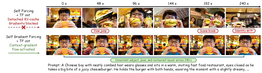
SF’s DMD losses update the shared DiT parameters \theta, so in general \mathsf{KV}_i^{0}(\theta_{r+1})\not\equiv\mathsf{KV}_i^{0}(\theta_r), yet no gradient signal tells \mathcal{C}_\theta how to write \tilde x_i into K/V such that later blocks denoise better. Over long horizons this manifests as view jumps, scene breaks, and identity drift.
Method
Self Gradient Forcing (SGF) is a two-pass training strategy that restores the missing memory-writing gradient without backpropagating through the serial rollout (which would be prohibitively deep for long videos).
Pass 1 — no-gradient rollout. Run the autoregressive causal generator exactly as at inference. At a randomly sampled block index and denoising exit step, record two things: the self-generated clean-latent context \{\tilde x_i\}_{i<j} used to populate the K/V cache, and the noisy latent z_j^t that the model was about to consume. No gradients are retained through this rollout.
Pass 2 — parallel context-gradient reconstruction. With the recorded exit-step inputs, re-run only that step in parallel. Treat the recorded context latents as stop-gradient clean inputs (sg[·]), but recompute the clean-context K/V representations \mathsf{KV}_{<j}^{0}(\theta) = \mathcal{C}_\theta(\text{sg}[\tilde x_{<j}], 0) and the causal attention from the current noisy block to those recomputed entries with gradients enabled. The DMD loss at z_j^t then flows through both the target-side denoising computation and the source-side cache-writing computation \mathcal{C}_\theta.
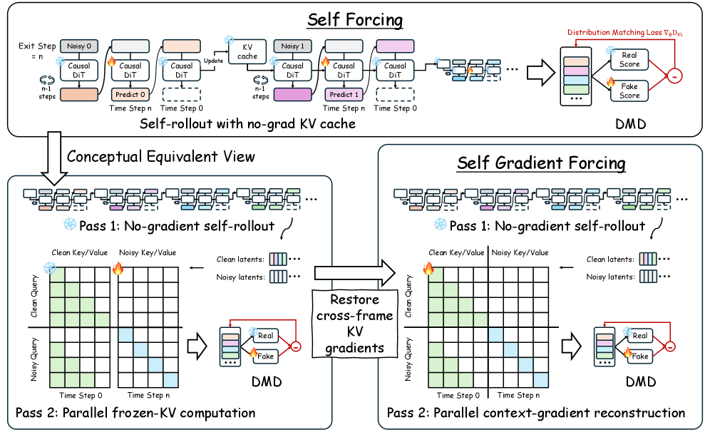
Because Pass 2 is a single parallel forward/backward over one exit step rather than an unrolled recurrence, memory cost is bounded by the sliding-window size, not by rollout length. Detaching \tilde x_{<j} prevents gradients from creeping back into earlier denoising trajectories; only the encoding of already-generated content into memory is supervised.
Experiments
All models share a fixed 5-second training window; 60s and 240s therefore probe native extrapolation. Every SGF vs SF comparison uses matched initialization, prompts, seeds, sink/FIFO policy, sliding window, chunking, and sampler — the sole variable is whether the exit-step loss reads a frozen cache (SF) or a gradient-reconstructed one (SGF). Two inference geometries are tested:
- Frame-wise: sink 4, total window 21, FIFO 16, current chunk 1.
- Chunk-wise: sink 3, total window 12, FIFO 6, current chunk 3, chunk size 3.
At 5s (VBench standard protocol), SGF and SF are broadly comparable across both geometries (Appendix B), confirming SGF does not degrade short-horizon quality. The main paper focuses on 60s (VBench-Long prompts) and 240s (128 MovieGen prompts), where memory-writing error compounds. Reported VBench-Long metrics are aesthetic quality, background consistency, dynamic degree, imaging quality, motion smoothness, subject consistency, and flickering, along with paired GSB human preference.
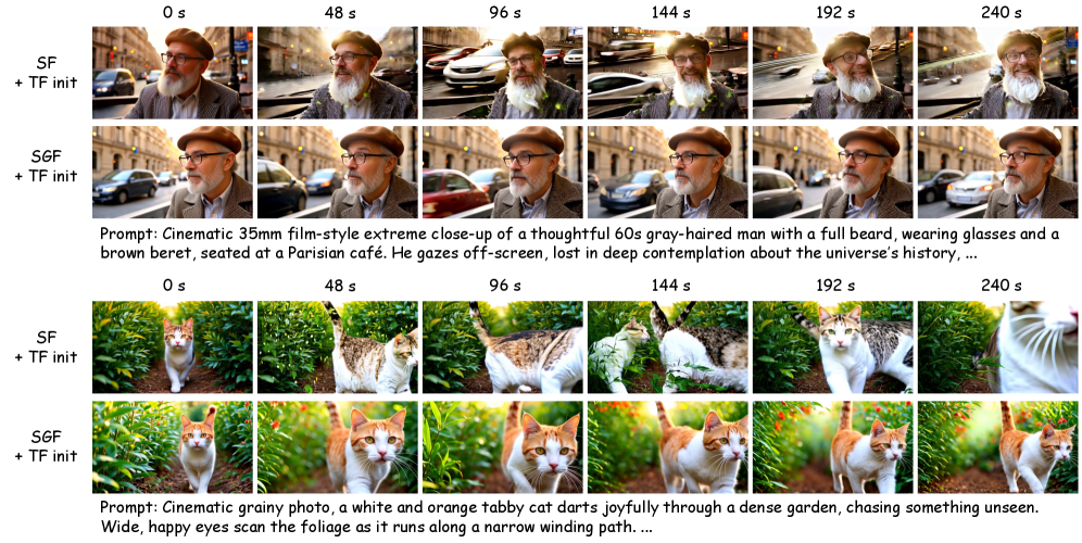
Qualitatively, the 240s frame-wise comparison shows SF producing scene cuts and identity drift while SGF maintains the same subject and background layout across the horizon, consistent with the hypothesis that supervising \mathcal{C}_\theta prevents drift in what the K/V cache actually stores.
Limitations and open questions
The abstract snippet does not disclose the absolute VBench-Long deltas, so the magnitude of improvement per metric is not verifiable from the excerpts provided here. Because gradients only reach one exit step per training example, the effective supervision on \mathcal{C}_\theta is stochastic over blocks; it is unclear how sample-efficient this is versus multi-step reconstruction. The stop-gradient on \tilde x_{<j} means SGF corrects how content is written to memory but not what content the earlier rollout produced — so failure modes that originate in the rollout itself (e.g., early-block hallucinations) are not directly addressed. Interaction with sink/FIFO policies, and whether the fix generalizes to very different chunk sizes or to models without a clean-context timestep, remain open.
Why this matters
Long-horizon autoregressive video is bottlenecked less by per-frame denoising than by what earlier generated frames leave in the K/V cache for later attention. SGF identifies that Self Forcing, despite training on self-generated histories, never supervises this memory-writing step, and closes the gap with a bounded two-pass scheme that avoids full rollout backprop. If the qualitative gains hold quantitatively, this is a cheap architectural-training fix that other causal video diffusion stacks can adopt directly.
Source: https://arxiv.org/abs/2607.20368
An Exam for Active Observers
Human vision is not a feed-forward classifier over a single retinal snapshot. Psychophysics has long distinguished a preattentive, parallel channel from serial, attention-demanding routines like curve tracing, exhaustive enumeration beyond the subitizing limit, and fine-grained cross-region comparison. These routines are executed through repeated gaze shifts and working-memory updates. Contemporary MLLM benchmarks, dominated by static VQA, do not distinguish between models that describe an image once and models that actually re-visit pixels. ActiveVision is a benchmark designed to force the latter, and it exposes a stark gap between frontier models and humans.
Task construction
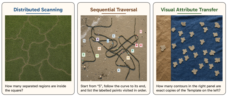
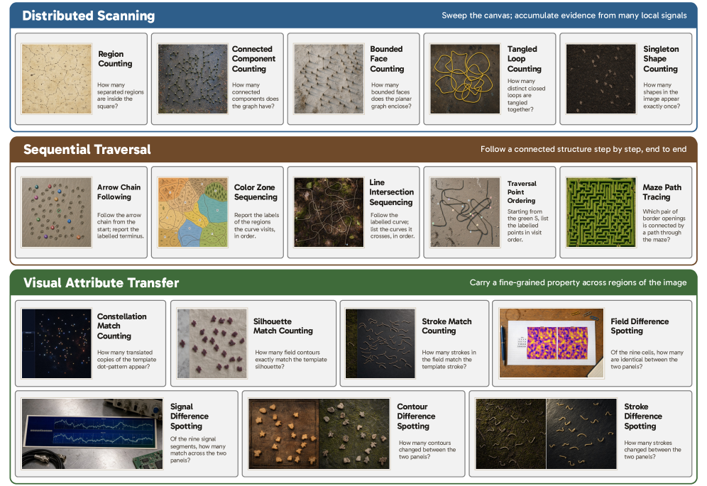
The benchmark comprises 17 procedurally generated tasks grouped into three families, each targeting one elemental active-vision operation:
- Distributed Scanning (5 tasks): counting spatially distributed local signals — dots, strokes, regions, graph faces, tangled loops. Failure modes are partial coverage (halted scans) and faulty individuation (merged or split signals).
- Sequential Traversal (5 tasks): following a connected structure — arrow chains, tangled curves through colored regions, maze paths, line-intersection sequences — while maintaining position, direction, and tally. Failure mode: gestalt interpolation, i.e. guessing the endpoint from the start.
- Visual Attribute Transfer (7 tasks): extracting a fine-grained property (length, curvature, thickness, dot pattern, orientation) from a reference region and matching it against candidates. Failure mode: prior substitution, applying a linguistic prior instead of measuring.
The key design principle is that each instance carries discriminative visual state whose information exceeds what any single language description can losslessly encode. This is enforced by a four-stage pipeline: a deterministic Python generator emits a geometric scaffold with ground truth (counts, ordered paths, matched attributes); a task-specific GPT-image-2 prompt re-renders the scaffold into a photorealistic image without altering positions, counts, or topology.
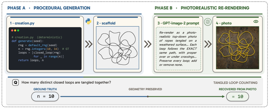
This decoupling matters: the ground truth is fixed by the scaffold, while the surface appearance is naturalistic enough to preclude solutions that exploit synthetic-image artifacts.
Evaluation and results
Each generator contributes N=5 instances, yielding 85 items. Scoring is exact-match on answers wrapped in <answer> tags, normalized for case and whitespace. Default protocol is pure CoT: one user message with question and image, no system prompt, no tools. Three human participants completed the full 85-item split via a self-paced web UI under the same criterion.
The headline result: at each model’s highest reasoning-effort tier, the best model — GPT-5.5 — solves 9/85 (10.6%) and scores 0/5 on 11 of the 17 tasks. Claude Fable 5, which tops reasoning and coding leaderboards, solves 3/85 (3.5%). Gemini 3.5 Flash reaches 7/85 (8.2%), Gemini 3.1 Pro 5/85 (5.9%), Claude Opus 4.7 4/85 (4.7%), Claude Opus 4.8 2/85 (2.4%). Humans average 81.7/85 (96.1%), with individual scores 97.6%, 96.5%, 94.1% — roughly 9\times the best model.
Two structural observations reinforce that this is not a single-model artifact. First, no item is solved by all six models, so success sets overlap only weakly. Second, an image-omitted control on GPT-5.5 scores 2/85 (2.4%), essentially matching the none-effort run with the image included — the ~10% ceiling therefore reflects genuine (if severely limited) visual work, not prompt priors leaking task structure. Average per-item reasoning budgets are substantial: 22.5k tokens for GPT-5.5, 15.4k for Claude Fable 5, 16.8k for Gemini 3.1 Pro, versus 33.6 s of wall-clock per item for humans.
Per-task granularity is informative. On Sequential Traversal, every model scores 0/5 on Traversal Point Ordering, Color Zone Sequencing, and Line Intersection Sequencing; only Maze Path Tracing and Arrow Chain Following get any hits, and no model exceeds 2/5 on any traversal task. On Visual Attribute Transfer, all four difference-spotting tasks are near-zero across models despite humans scoring \geq 4.3/5. Distributed Scanning shows the only isolated bright spots: GPT-5.5 gets 2/5 on Region Counting and 3/5 on Constellation Match Counting, while Tangled Loop Counting is 0/5 for every model.
Limitations and open questions
The evaluation split is small (N=5 per task, 85 total) which increases variance on per-task cells, though the aggregate pattern is unambiguous. The authors report that agentic tool use — letting the model write and run its own vision code — does not close the gap, because such code is unreliable on realistic imagery and catching its failures itself requires active perception. This suggests the bottleneck is not a missing external tool but the absence of a closed perception-action loop within the model. It is unclear whether this is fundamentally an architectural issue (no mechanism to re-fixate or maintain a visual scratchpad) or a training-distribution issue (no supervision incentivizes serial visual routines). The photorealistic rendering step also introduces some coupling to GPT-image-2’s failure modes, though ground truth is preserved by construction.
Why this matters
ActiveVision isolates a capability — serial, attention-guided re-inspection of pixels — that current MLLMs essentially lack, and it does so with tasks a child can perform. A \sim 10\% ceiling against a 96\% human baseline on a benchmark that already accounts for prompt priors indicates that scaling reasoning-token budgets over static image embeddings will not close this gap; a mechanism for iterative visual access is needed.
Source: https://arxiv.org/abs/2607.16165
Beyond Euclidean Clipping: Overcoming Exploration Collapse in LLM RL via Riemannian Isometric Policy Optimization
Problem
PPO-Clip and its LLM-era descendants (GRPO, DAPO, GSPO, GMPO, DCPO) constrain the importance ratio r_{s,a}(\theta) = \pi_\theta(a|s)/\pi_{\theta_{\text{old}}}(a|s) to lie in (1-\epsilon, 1+\epsilon). The authors argue this is geometrically wrong: the ratio is a Euclidean quantity, but policies live on a Riemannian manifold whose local metric is the Fisher information (equivalently, the second-order expansion of KL). Under a uniform Euclidean clip, the KL “budget” consumed by an update depends strongly on \pi_{\theta_{\text{old}}}(a|s).
Concretely, with \epsilon=0.2: a high-probability token at \pi_{\text{old}}=0.8 can move to 0.96 (change +0.16), while a low-probability token at \pi_{\text{old}}=0.01 can only reach 0.012 (change +0.002). The two updates consume drastically different geometric distances (0.016 vs. 0.0002 in the paper’s units). The result is that already-exploited tokens are amplified freely while rare-but-valuable tokens are effectively frozen — exploration collapse. DAPO’s Clip-Higher (\epsilon_{\text{high}}=0.28) only raises the low-prob cap to 0.0128 (a +0.0008 delta), while simultaneously letting high-prob tokens saturate to 1.0, worsening the imbalance.
Method: Riemannian Isometric Clip
RIPO replaces the constant Euclidean \epsilon with a per-token clip radius derived from requiring equal geometric distance under the local Fisher metric. Using the second-order KL expansion, the authors define
d_{\text{geom}}(\pi_{\theta_{\text{old}}}, \pi_\theta) \triangleq \tfrac{1}{2}\pi_{\theta_{\text{old}}}(a|s)\,(r_{s,a}(\theta)-1)^2 \le \delta.
Solving for the ratio gives a distribution-dependent clip:
|r_{s,a}(\theta) - 1| \le \epsilon_{s,a}(\pi_{\theta_{\text{old}}}), \qquad \epsilon_{s,a}(\pi_{\theta_{\text{old}}}) = \sqrt{\frac{\delta}{\pi_{\theta_{\text{old}}}(a|s)}}.
Every token consumes the same trust-region budget \delta. Revisiting the earlier example with \delta=0.02: the \pi_{\text{old}}=0.8 token is now capped at 0.92 (tighter than PPO’s 0.96), while the \pi_{\text{old}}=0.01 token can reach 0.024 — a 2\times increase in permissible update relative to PPO-Clip. Both consume the same geometric distance 0.01.
Practically this is a drop-in replacement inside the standard GRPO-style surrogate: compute \epsilon_{s,a} from the detached old-policy probabilities per token, then apply the usual \min(r\hat A, \text{clip}(r, 1-\epsilon_{s,a}, 1+\epsilon_{s,a})\hat A). The authors also permit asymmetric \{\delta_{\text{low}}, \delta_{\text{high}}\} (analog of Clip-Higher, but in geometric units). Following common practice they retain a dual clip at [0.5, 10] to bound extreme ratios, drop the KL penalty, and use group-relative advantages. Default \delta = 0.05.
The paper further argues RIPO enjoys a better bias–variance profile: since the clip radius scales as 1/\sqrt{\pi_{\text{old}}}, low-probability tokens (which contribute high-variance importance-sampling terms) get proportionally larger but geometrically bounded updates, while high-probability tokens are dampened.
Results
Across seven competition-level math benchmarks and four base models (Llama3.2-3B-Instruct, Qwen3-1.7B/4B/8B-Base), RIPO outperforms GRPO, DAPO, GSPO, GMPO, and DCPO. The headline number is up to 60\% improvement over GRPO on AIME24.
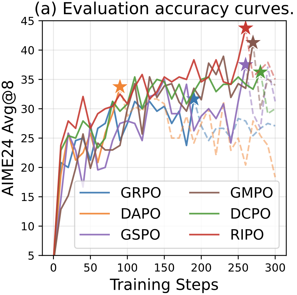
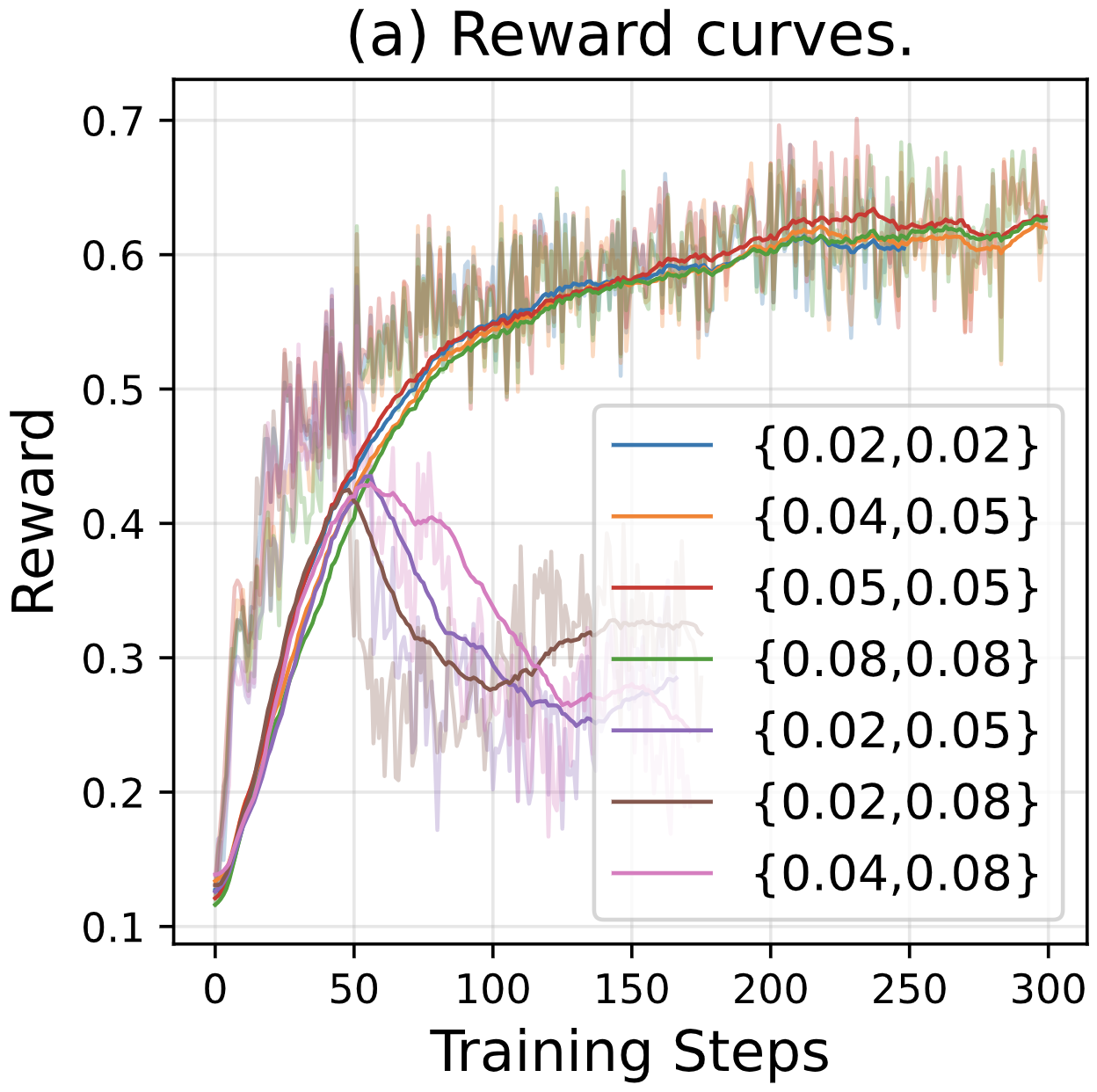
The AIME accuracy curves on Qwen3-8B show that Euclidean-clip baselines plateau early — the signature of exploration collapse — whereas RIPO continues to improve. On smaller models the mechanism is even clearer: on Qwen2.5-1.5B-Instruct trained on GSM8k, RIPO’s asymmetric geometric clip yields a monotonically rising accuracy trace where PPO-style methods stall or oscillate.
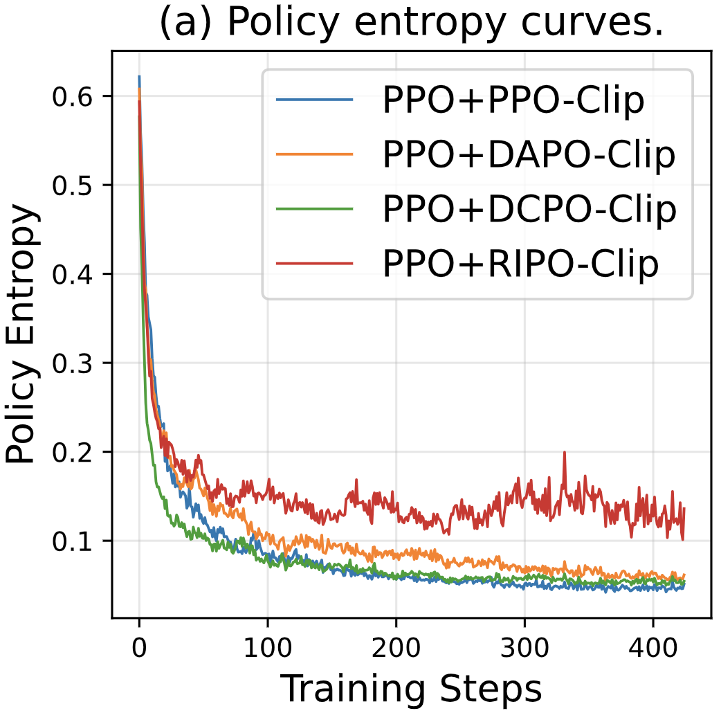
The \{\delta_{\text{low}}, \delta_{\text{high}}\} ablation confirms the exploration/exploitation lever: larger \delta_{\text{high}} (more upward budget on rare tokens) accelerates learning, while \delta_{\text{low}} controls how aggressively already-preferred tokens can be pushed down.
Limitations and open questions
- The geometric distance d_{\text{geom}} is a second-order Taylor surrogate for KL. It is accurate near r=1 but degrades for the very large ratios that low-probability tokens can now legally reach (e.g., \epsilon_{s,a}=\sqrt{\delta/0.001}\approx 7 at \delta=0.05), which is precisely why the [0.5, 10] dual clip is retained. The interaction between the isometric bound and the dual clip is not analyzed.
- All experiments use group-relative advantages on math benchmarks; behavior on general RLHF preference tasks, tool-use, or long-horizon agentic RL is untested.
- \pi_{\theta_{\text{old}}}(a|s) is taken from the sampling policy; the treatment under multi-step off-policy or replay is not discussed.
- No comparison against natural-gradient or K-FAC style methods, which target the same geometric issue from the optimizer side rather than the clip side.
- The AIME24 “60\% improvement” is relative; absolute numbers per benchmark are not extractable from the sections provided.
Why this matters
Clipping in LLM RL has accreted a stack of heuristics (Clip-Higher, sequence-level, geometric-mean, dynamic-adaptive) all patching the same underlying geometric mismatch. RIPO identifies the cause — Euclidean thresholds on a Fisher-Riemannian manifold — and fixes it with a one-line, per-token clip radius \sqrt{\delta/\pi_{\text{old}}} that is trivial to add to any GRPO/DAPO codebase.
Source: https://arxiv.org/abs/2607.10169
SLPO: Scaling Latent Reasoning via a Surrogate Policy
Problem
Reinforcement learning with verifiable rewards (RLVR) has become the standard tool for eliciting test-time scaling in explicit chain-of-thought (CoT) reasoners, but the compute cost is dominated by decoding every intermediate step as a language token. Latent reasoners (COCONUT, CODI, CoLaR) instead propagate reasoning as continuous hidden states and reach comparable accuracy at much shorter horizons. However, they remain trained by imitation of teacher CoT: (i) continuous latent transitions have no tractable per-step likelihood usable in a PPO-style objective, and (ii) fixed thinking budgets preclude adaptive stopping, so outcome rewards cannot select trajectory length. Consequently, latent reasoners cannot yet exploit test-time scaling in the way explicit CoT does.
SLPO addresses both gaps: it defines an empirical surrogate density over latent transitions for policy-gradient credit assignment, and adds a learned stopping head that is first cold-started against correctness and then jointly refined by outcome-reward RL.
Method
Stage 1 — Stopping-gate cold start. A stopping head g_\theta is attached on top of latent state h, producing s_\theta(h)=\sigma(g_\theta(h)), the probability of terminating latent computation at that step. For each input x_i, the frozen latent backbone samples N stochastic latent trajectories up to T_{\max}. For every trajectory n and every candidate stopping length t\in[T_{\min},T_{\max}], the model decodes an explicit answer conditioned on the prefix h_{i,1:t}^{(n)}:
a_{i,n,t}\sim \pi_\theta(\cdot\mid x_i, h_{i,1:t}^{(n)}).
Correctness under the verifiable reward defines the valid-stopping set \mathcal{V}_i^{(n)} = \{t : R(a_{i,n,t}, a_i^\star)=1\}. Writing \rho_{i,n,t}=s_\theta(h_{i,t}^{(n)}), the induced stop-time distribution is
P_\theta(\tau_i^{(n)}=t) = \rho_{i,n,t}\prod_{k<t}(1-\rho_{i,n,k}),
and the head is trained by maximizing total mass on valid stopping times:
\mathcal{L}_{\text{stop}}^{(i)} = -\frac{1}{N}\sum_{n=1}^N \log \sum_{t\in \mathcal{V}_i^{(n)}} P_\theta(\tau_i^{(n)}=t).
This introduces a continue-vs-stop interface with well-defined likelihood before any RL fine-tuning.
Stage 2 — Surrogate policy optimization. The core difficulty is that a continuous transition h_{t-1}\to h_t has no closed-form density under a deterministic recurrence, so a surrogate is estimated empirically by resampling K latent successor states from the (stochastic, e.g. MC-dropout) backbone and forming a transition-likelihood surrogate that can be plugged into an outcome-reward objective. Verifiable rewards then weight the joint log-likelihood of (a) the surrogate latent transitions, (b) the decoded answer tokens, and (c) the gate’s stop-time distribution:
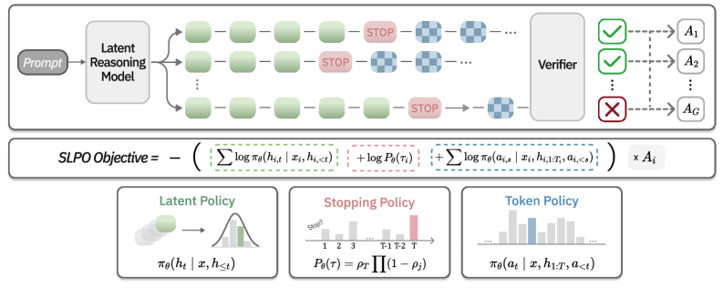
Because the gate participates in the objective, correctness signals not only shape latent transitions but also reallocate compute across steps, producing a variable-horizon policy from a fixed-budget backbone. RLOO and GRPO are both compatible advantage estimators.
Inference. At test time, latent thinking rolls forward while the gate samples stop-vs-continue; once stopped, the answer is decoded conditioned on the terminating latent prefix. Parallel sampling yields Pass@k curves.
Results
Evaluation is on GSM8K-Aug training with held-out GSM8K-Test, GSM-Hard, and MultiArith, using both GPT-2 (124M) and Llama-3.2-1B backbones for COCONUT and CODI. Deterministic accuracy uses no dropout; Pass@k uses MC-dropout p=0.1.
On GPT-2, COCONUT+SLPO improves average Acc from 40.88 to 42.13 and Pass@16 from 50.86 to 52.22. CODI+SLPO gains are similar on average Acc (47.59 → 47.66) but larger on Pass@16 (54.81 → 55.84). On Llama-3.2-1B the gains are more pronounced for the weaker COCONUT backbone: average Acc 22.29 → 25.01 and Pass@16 37.06 → 41.38, with GSM-Hard Pass@16 lifting 9.94 → 10.93 and MultiArith Pass@16 63.10 → 71.38. CODI+SLPO on Llama moves Pass@16 from 60.63 to 62.18, with GSM8K Pass@16 rising 67.48 → 70.28. Pass@k gains consistently exceed Acc gains, consistent with the interpretation that outcome-reward RL sharpens the stochastic latent policy rather than the deterministic mode.
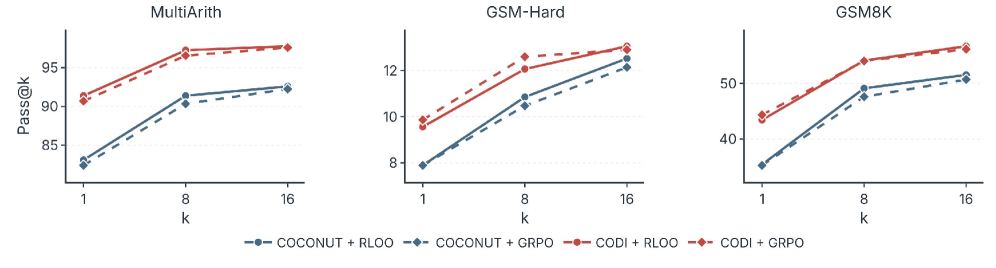
RLOO and GRPO variants are close on CODI but RLOO tends to dominate on COCONUT at higher k, suggesting that lower-variance leave-one-out baselines help when the underlying latent policy is weaker.
Hyperparameter sensitivity. Group size G (trajectories per problem) dominates K (surrogate-estimation samples per transition). Sweeping each over \{2,4,8\} with the other fixed at 4, larger G consistently improves Pass@2 on GSM-Hard and MultiArith, while K saturates once large enough to stabilize the surrogate density. This is the expected pattern: K controls estimator variance for a nuisance quantity, G controls advantage-estimation variance for the true policy gradient.
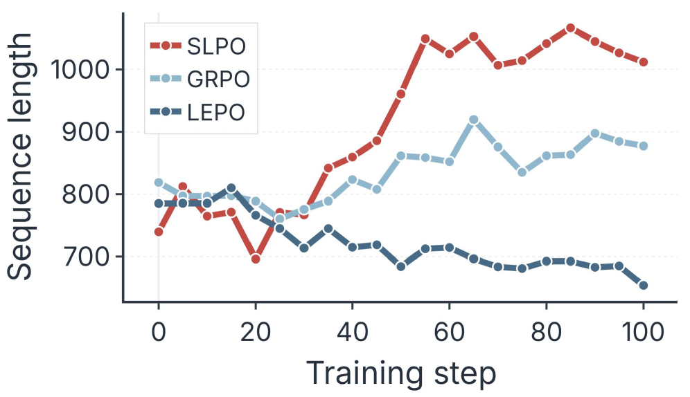
Adaptive length. In the soft-token transfer setting on Llama-3.2-1B, outcome-reward optimization changes mean generated sequence length over training, showing that the gate is doing nontrivial compute allocation rather than collapsing to a single horizon:
Limitations and open questions
Evaluation is confined to grade-school arithmetic plus a limited soft-latent transfer to MATH500/AIME25/AMC23; whether the surrogate remains well-behaved on longer-horizon, higher-branching reasoning (theorem proving, code) is unresolved. The surrogate density relies on MC-dropout stochasticity for its resampling — deterministic latent backbones would need an alternative noise source. Gains on strong deterministic accuracy are small (often <1 point); most of the benefit lives in Pass@k, which raises the question of whether the RL is teaching new reasoning or reweighting an existing distribution of latent modes. Finally, the two-stage decoupling (cold start then RL) leaves open whether the gate and surrogate can be trained fully jointly from scratch.
Why this matters
SLPO is the first demonstration that outcome-reward RL — the mechanism behind explicit-CoT test-time scaling — can be applied to autoregressive latent reasoners without a per-step token likelihood, by combining an empirical transition surrogate with a learned stopping distribution. If the surrogate approach generalizes beyond arithmetic, it removes the main technical barrier separating latent reasoning from the RLVR-driven scaling curves that now dominate explicit CoT.
Source: https://arxiv.org/abs/2607.19691
SLAI T-Rex: Full-Parameter Post-training of the DeepSeek-V4 Family on Ascend SuperPOD
Problem
Full-parameter post-training of trillion-scale MoE models is bottlenecked by three system-level pathologies: (1) memory pressure from optimizer states, activations, and expert weights that exceed per-device HBM even at high parallelism; (2) exposed communication — all-to-all dispatch/combine for MoE routing and tensor-parallel all-reduces that do not naturally overlap with compute; and (3) kernel inefficiency from fragmented ops in attention, MoE gating, and expert GEMMs. Most published recipes target NVIDIA GPUs with NCCL/NVLink. This report instead builds an end-to-end stack on Huawei Ascend NPU SuperPOD for the DeepSeek-V4 family, addressing an underexplored question: what MFU is realistically achievable for trillion-parameter MoE post-training on non-GPU accelerators, and where do the bottlenecks shift?
Method
The system is organized as a three-layer hierarchical optimization spanning parallelism, orchestration, and kernels.
Parallelism. The authors combine expert parallelism (EP), pipeline parallelism (PP), tensor parallelism (TP), and ZeRO-style optimizer sharding, chosen to fit the DeepSeek-V4 MoE topology (fine-grained experts with shared experts) onto Ascend SuperPOD’s interconnect. The choice is guided by minimizing exposed all-to-all volume relative to the HCCL fabric bandwidth, i.e. keeping EP groups inside high-bandwidth domains and pushing PP across lower-bandwidth links. For an MoE layer with E experts, top-k routing, hidden h, and per-token expert count k, dispatch volume per token per step scales as O(k h), so the EP group size |EP| is picked so that
T_{\text{a2a}} \approx \frac{k h B}{|EP| \cdot BW_{\text{intra}}}
remains smaller than the corresponding expert GEMM time.
Computation-communication orchestration. All-to-all dispatch/combine is split into micro-chunks and interleaved with the shared-expert MLP and attention compute of neighboring micro-batches, so that the effective step time approaches \max(T_{\text{comp}}, T_{\text{comm}}) rather than their sum. Pipeline schedules use a 1F1B-like variant with warm-up shaping tuned so that PP bubble time is amortized across the MoE dispatch latency; combined with recomputation policies applied selectively to attention (not to MoE experts, whose activations are cheaper to store than to recompute given routing sparsity), this pushes peak activation memory below the per-NPU HBM ceiling.
Kernels. At the low level, the team fuses attention (FlashAttention-style tiled softmax with online normalization), MoE gating + permutation + unpermutation, and grouped GEMMs for expert forward/backward. Grouped GEMM is critical because per-expert token counts n_e are highly imbalanced; a padded batched GEMM wastes FLOPs proportional to \max_e n_e / \bar{n}_e, whereas the grouped variant executes one kernel launch over a jagged batch. Numerical stability under bf16 is preserved by keeping master weights and optimizer moments in fp32 with loss-scaled reductions.
Results
The headline number is 34.22% MFU on the DeepSeek-V4-Flash workload on Ascend SuperPOD, a 2.93× improvement over the open-source baseline recipe on the same hardware. This is in the same ballpark as reported MFUs for trillion-scale MoE training on H100/H800 clusters (typically 30–40% depending on sequence length and routing), which is the more meaningful comparison — it demonstrates that with sufficient co-design the accelerator choice is not the binding constraint. Training stability is maintained across the run, i.e. no divergence or loss spikes requiring rollback, which is nontrivial for full-parameter (not LoRA) post-training of a trillion-parameter MoE where router collapse and expert imbalance are known failure modes.
On top of the optimized infrastructure, the authors build a CPT + SFT workflow for Operations Research tasks. The data pipeline mixes collected OR domain corpora with solver-verified synthetic optimization documents — problems where a classical solver (LP/MILP/CP) produces a ground-truth optimum that is used both to filter synthetic problem statements and to label chain-of-thought derivations. The abstract reports a resulting dataset of ~10K high-quality examples (truncated in the provided text). This is a defensible synthetic-data recipe: solver verification removes the main hazard of LLM-generated math training data, namely plausible but incorrect intermediate steps.
Limitations and open questions
The report is a systems paper first; the OR downstream evaluation is not detailed in the provided abstract, so it is unclear how much the CPT+SFT stage improves solve rates on standard OR benchmarks (NL4Opt, ComplexOR, MAMO) versus the base DeepSeek-V4-Flash. The 34.22% MFU is impressive but still leaves roughly two-thirds of theoretical FLOPs on the table; the breakdown between residual communication exposure, kernel inefficiency, and pipeline bubbles is not quantified here. Generalizability of the parallelism recipe to other MoE topologies (denser routing, larger k, or non-shared-expert designs) is not established. Finally, reproducibility outside Ascend SuperPOD is limited by dependence on HCCL and vendor kernels; the techniques transfer conceptually to GPU clusters but the specific overlap schedules would need retuning.
Why this matters
This is one of the few public, detailed accounts of full-parameter post-training of a trillion-parameter MoE on non-NVIDIA hardware reaching competitive MFU, which matters both for the practical question of accelerator diversity in frontier training and as a concrete recipe for MoE communication-computation overlap that is applicable beyond Ascend. The solver-verified OR data pipeline is also a reusable template for domains where correctness of synthetic training data can be mechanically checked.
Source: https://arxiv.org/abs/2607.20145
Beyond Relevance-Centric Retrieval: Rubric-Oriented Document Set Selection and Ranking
Problem
Retrieval evaluation is stuck in a per-document paradigm: nDCG and its relatives score documents independently against a relevance judgment and aggregate linearly. When the downstream consumer is an LLM performing RAG or agentic reasoning, what matters is the joint utility of the returned set — whether the documents contradict each other, duplicate content, or collectively cover the reasoning chain needed to answer the query. The authors give a concrete example where nDCG@5 = 100% yet the set contains factual conflict between Doc [11] and [12], redundancy across pairs, and missing key facts.
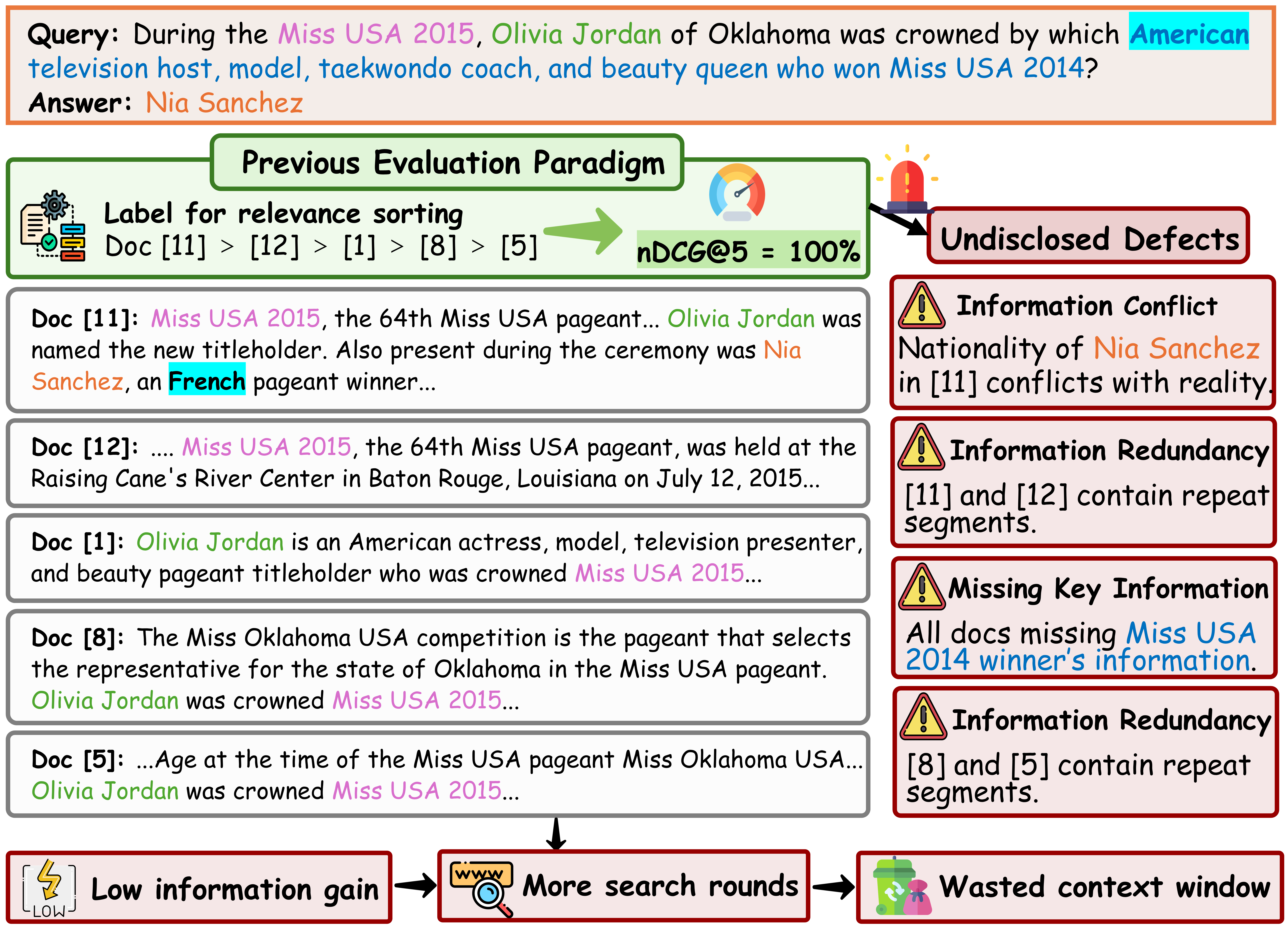
This is the gap the paper targets: build an evaluator that scores document sets along interaction-sensitive dimensions, diagnose where current rerankers fail, and use those same rubrics as a training-free selection signal.
Method
SetwiseEvalKit organizes evaluation into a three-level, nine-dimension taxonomy — document-level, set-level, and global-level — with ~28K rubrics spanning short-form and long-form scenarios. The set-level dimensions explicitly capture cross-document interactions (redundancy, conflict, complementarity), and the global level captures whether the set is sufficient to reconstruct the answer (reachability, coverage).
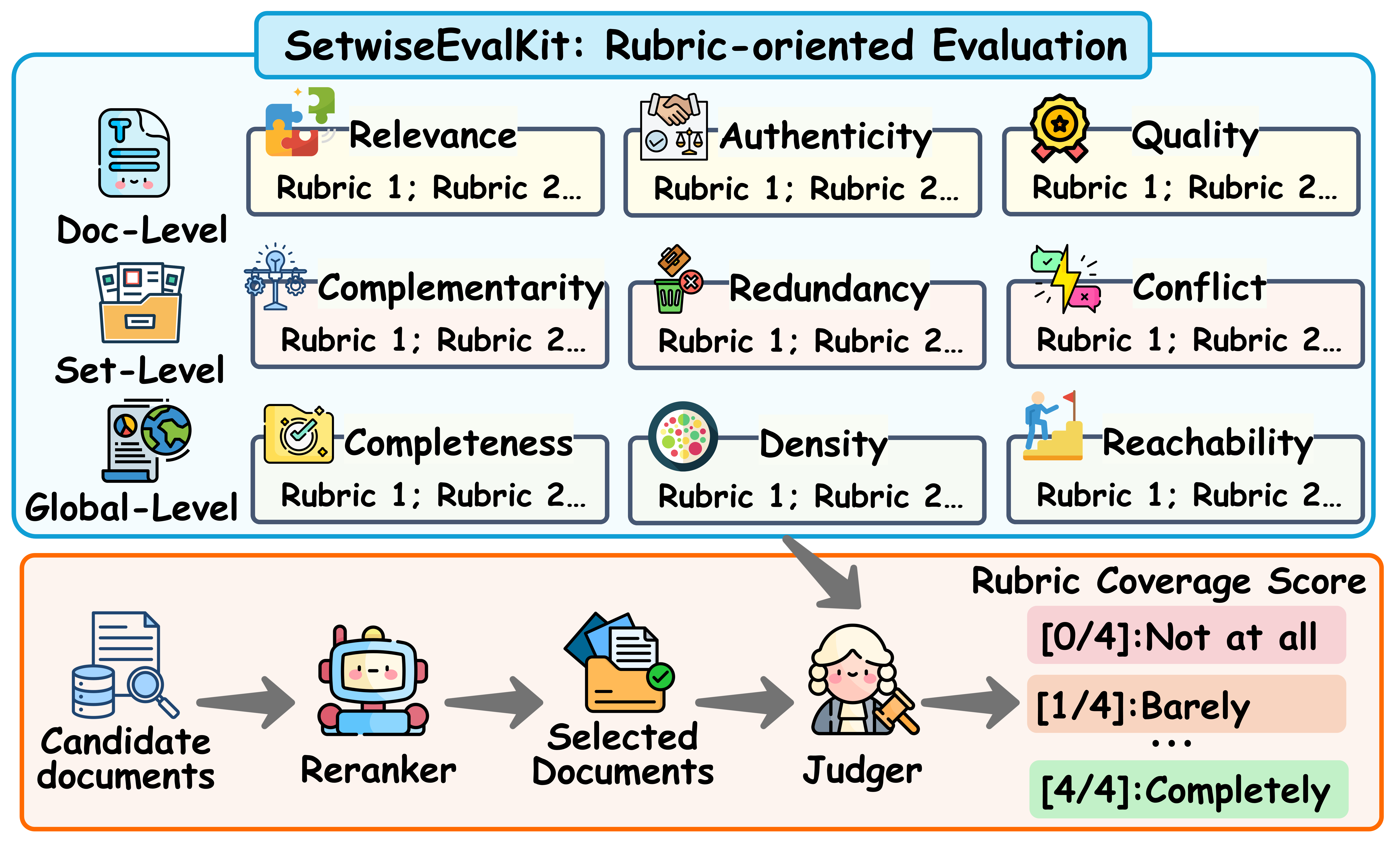
Formally, given query q and reference answer a, they synthesize \mathcal{R}=\{r_1,\ldots,r_K\} conditioned on (q,a). A reranker m returns S_m\subseteq\mathcal{C} with |S_m|\le k. The judge produces
\text{Score}(S_m) = \mathcal{E}(q, S_m, \mathcal{R}) \in \mathbb{R}^9,
i.e., the LLM reads the entire set once and grades each dimension on 0–4. Because rubrics are conditioned on the reference answer, they encode the information need at a granularity that reveals set-level pathologies — e.g., the case study query yields Redundancy 2/4 and Conflict 2/4 because multiple documents make contradictory “crowning” claims, and Reachability 1/4 because the reasoning chain cannot be reconstructed even though surface relevance is high.
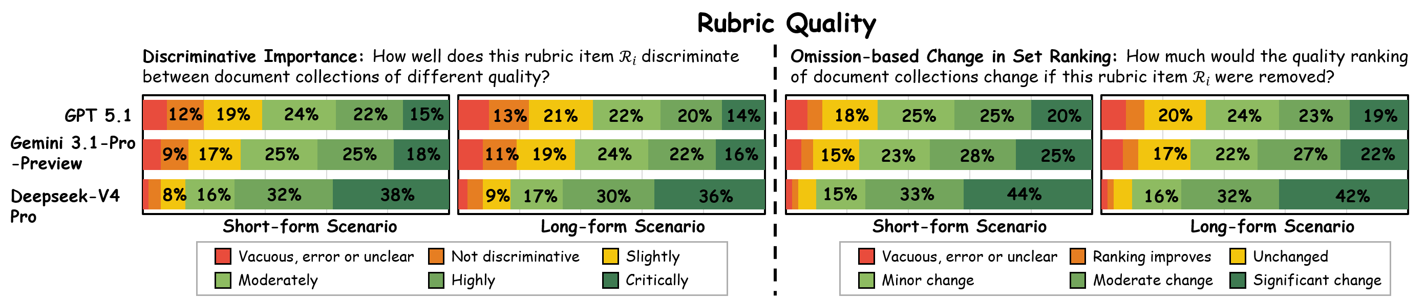
Human validation (Figure 3) shows Ph.D. raters find the generated rubrics of high quality, supporting the use of the rubric bank as a benchmark rather than a noisy LLM artifact.
Rubric4Setwise turns the same rubrics into a selection signal at inference time. Rather than scoring documents in isolation, it scores candidate subsets against \mathcal{R} and picks the subset maximizing rubric coverage. It is training-free: the rubric generator and the set scorer are both prompted LLMs, and selection is a greedy/beam procedure over the candidate pool. The key inductive bias is that the same rubric distribution that defines “good set” for evaluation is the correct objective for selection — matching evaluator and selector removes the specification gap that plagues nDCG-trained rerankers.
Results
The authors benchmark 12 rerankers spanning three families: ad-hoc cross-encoders and listwise LLM rankers (BGE-Reranker-Large, MonoT5, RankT5, RankLlama, RankVicuna, RankZephyr, Setwise), reasoning-enhanced rerankers (Rank1, Rearank, ReasonRank), and setwise rerankers (SetR, Rank4Gen), plus BM25 and Google Search lower bounds.
Headline findings from Section 4:
- Ceiling is low. The best reranker achieves ≤45% rubric coverage. Under a rubric evaluator, current systems leave the majority of set-level quality on the table.
- Cross-document coordination is uniformly weak. Redundancy, conflict, and complementarity dimensions are the lowest-scoring across all 12 rerankers. Even setwise-trained methods (SetR, Rank4Gen) do not close this gap meaningfully.
- No cross-regime winner. Rankers that lead in short-form contexts drop in long-form, and vice versa — evidence that relevance-optimized objectives do not generalize across set-composition regimes.
- Rubric4Setwise wins downstream generation with fewer documents and fewer search rounds, and is reported as the only method to consistently do so — matching evaluator and selector via shared rubrics is empirically the right coupling.
The Section 5 case study makes the failure mode concrete: traditional metrics rate the set perfectly, while Redundancy 2/4, Conflict 2/4, and Reachability 1/4 flag exactly the deficiencies a downstream generator would trip over.
Limitations and open questions
- The evaluator \mathcal{E} is itself an LLM; systematic biases in the judge propagate into both benchmark rankings and Rubric4Setwise’s selection signal. The human validation covers rubric quality but not judge scoring calibration on adversarial sets.
- Rubric generation requires a, the reference answer. In deployment there is no reference — the selection-time procedure must synthesize rubrics from q alone or from a preliminary draft, and the paper’s evaluation of Rubric4Setwise conflates these regimes with the reference-conditioned benchmark.
- Compute cost is not the focus, but subset scoring with an LLM is combinatorial; scaling behavior with |\mathcal{C}| and k is not fully characterized.
- The nine dimensions are motivated but not shown to be minimal or orthogonal; dimension collapse or reweighting could change the ranking of methods.
Why this matters
If LLMs are the primary consumer of retrieval, the evaluation target should be joint set utility, not pointwise relevance — and this paper shows the gap is large (≤45% coverage for the best of 12 rerankers) and that using rubrics as both evaluator and selector closes it without training. Expect rubric-conditioned set selection to displace pointwise reranking as the default RAG frontend.
Source: https://arxiv.org/abs/2607.19747
Scaling Laws for Hypernetwork-Based Knowledge Injection in Large Language Models
Problem
Reliable, large-scale knowledge injection into frozen LLMs remains unsolved: fine-tuning is expensive and destructive, RAG shifts the burden to retrieval, and in-context learning scales poorly with the number of facts. This paper studies whether a hypernetwork — trained once on a large fact corpus — can produce a LoRA adapter that, when spliced into a frozen target LM, makes it answer questions about arbitrary facts drawn from that corpus. The novel angle is empirical: hypernetworks have not been characterized under a scaling-laws lens, and prior applications entangled hypernetwork capacity with target model capacity. Here the target LM is frozen, so the hypernetwork’s scaling behavior is isolated.
Method
The setup treats knowledge injection as amortized adaptation. Each training example is a query q together with a set \mathcal{F} = \{f_1, \dots, f_N\} \subset \Omega of N verbalized facts, exactly one of which is relevant; the remaining N-1 are uniform negatives from the fact corpus \Omega. A hypernetwork H_\phi(\mathcal{F}) outputs a fixed LoRA adapter \Delta\theta inserted into the frozen target model \mathcal{M}_\theta, and the training loss is the standard autoregressive NLL of the answer a under \mathcal{M}_{\theta + \Delta\theta}. Only \phi is updated; \theta is never touched. Default N=4.
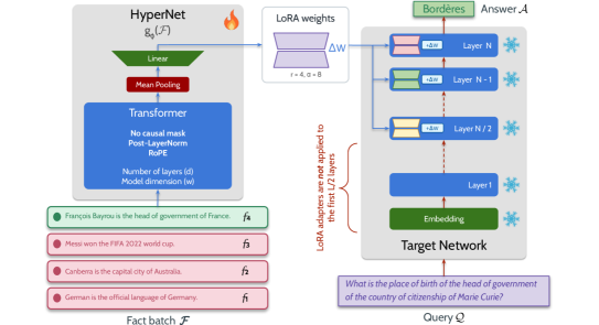
The training corpus is MegaWikiQA, built from Wikidata5M (4.6M entities, 822 relations, 22M triplets). Multi-hop QA examples for k \in \{1,2,3,4\} are generated by uniform random walks in the KG. A recursive grammar f converts a k-hop walk (s_1, r_1, o_1, \dots, r_k, o_k) into a nested noun phrase (e.g., “the country of citizenship of the spouse of Marie Curie”), which is then wrapped into a question template. Because the walks are deterministic in the KG, ground-truth answers are unambiguous, and the dataset spans 39 knowledge domains — enough to hold out entire domains for OOD evaluation.
Four evaluation metrics probe distinct generalization axes: ID validation loss, OOD non-rephrased loss (held-out domains, same templates), OOD rephrased loss (paraphrased questions on held-out domains), and OOD MCQ (multiple-choice reformulation on held-out domains). All scaling fits use \mathcal{L} = a x^b estimated by least-squares in log-log space on final-epoch loss. The target model is Qwen2.5-1.5B-Instruct in the width/depth/fact-count sweeps, selected because the Qwen2.5 family provides consistent architectures across a wide size range.
Results
Width scaling. Varying d_{\text{model}} \in \{64, 128, 256, 512, 1024\} at fixed depth yields clean power laws on all four metrics.
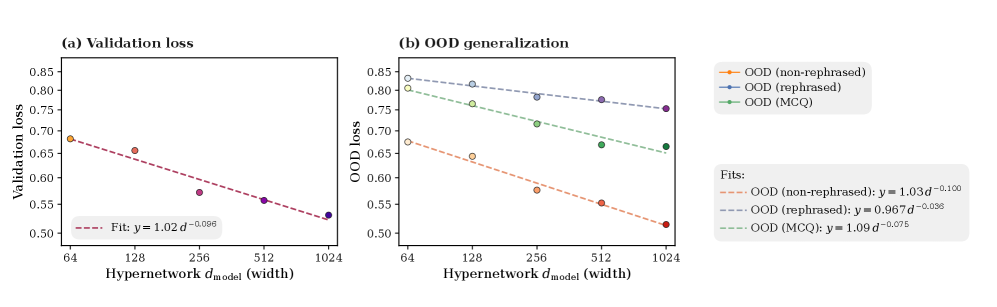
- ID validation: \mathcal{L}_{\text{val}} = 1.02 \cdot d^{-0.096}
- OOD non-rephrased: exponent -0.100
- OOD rephrased: exponent -0.036
- OOD MCQ: exponent -0.075
The near-equality of the ID exponent (-0.096) and the OOD non-rephrased exponent (-0.100) shows that width buys in-distribution and same-template OOD recall at essentially the same rate. But the rephrased exponent (-0.036) is roughly 2.7× flatter, indicating width alone does not confer robustness to surface-form variation — a capability that likely requires either more diverse training paraphrases or a mechanism beyond raw parameter count. MCQ falls in between (-0.075), consistent with a moderate distribution shift from open-ended generation.
Depth scaling. Varying the number of hypernetwork transformer layers L_{\text{HN}} at fixed width:
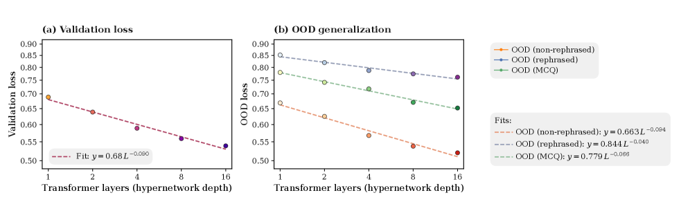
- ID validation: \mathcal{L}_{\text{val}} = 0.677 \cdot L^{-0.088}
- OOD non-rephrased: exponent -0.096
- OOD rephrased: exponent -0.042
The depth exponents track the width exponents closely (ID -0.088 vs -0.096; OOD non-rephrased -0.096 vs -0.100; OOD rephrased -0.042 vs -0.036). Depth and width thus appear roughly interchangeable for injection quality, and — importantly — the rephrasing gap persists: whichever axis you scale, robustness to linguistic reformulation improves only weakly. This is a structural, not architectural, bottleneck.
Limitations and open questions
The exponents are all shallow (magnitudes \le 0.1), so halving loss requires roughly two orders of magnitude in hypernetwork parameters — expensive relative to alternatives like retrieval. The rephrased-OOD floor suggests the hypernetwork may be learning template-conditioned pattern matching rather than genuine fact-content routing; the paper does not disentangle whether this is a data-diversity issue or an architectural one. Only Qwen2.5-1.5B is the default target; joint scaling of target and hypernetwork is deferred. The random-walk QA generation may also over-represent short, chain-like reasoning patterns and under-represent lateral compositions. Finally, N=4 facts is small compared to realistic retrieval buffers, and the reported fact-count sweep is not shown here.
Why this matters
This is the first controlled scaling study of hypernetworks as a knowledge-injection substrate for frozen LLMs, and it establishes that both width and depth follow clean, if shallow, power laws — while exposing a robust generalization gap under paraphrasing that neither axis meaningfully closes. That gap is the key research target for anyone hoping hypernetworks can eventually replace or complement RAG.
Source: https://arxiv.org/abs/2607.19604
Hacker News Signals
Gemini 3.6 Flash, 3.5 Flash-Lite, and 3.5 Flash Cyber
Google released three model variants targeting different cost/capability points. Gemini 3.6 Flash is positioned as the primary upgrade: it claims to match 2.5 Pro on several benchmarks while running at Flash-class latency and cost. The architectural specifics are undisclosed, but the announced 1M-token context window is retained and the model is multimodal (text, image, audio, video, code). The benchmark claims include MMLU, GPQA, and coding evaluations, though Google’s own numbers should be read against the usual self-reported-benchmark caveats.
Gemini 3.5 Flash-Lite is the aggressive cost-reduction play: priced below 3.5 Flash with the intent of replacing it for high-throughput, latency-sensitive pipelines where per-token cost dominates. It is the smallest member of the family still supporting the full multimodal input set.
Gemini 3.5 Flash Cyber is a fine-tuned variant explicitly trained for security use cases — CTF challenges, vulnerability analysis, exploit reasoning. Google is positioning it alongside CyberSecEval-style benchmarks. Specialized security fine-tunes have proliferated (see also Mistral’s codestral family), and this follows the pattern of a general base model with domain-specific RLHF or SFT on security corpora.
The release strategy reflects the industry shift toward model families rather than single flagship releases: developers pick a point on the cost-latency-capability Pareto frontier. The Flash line competes directly with Anthropic’s Haiku and OpenAI’s 4o-mini tier.
Notable omission: no public technical report accompanies the release. Architectural details (depth, width, MoE vs. dense, training compute) remain opaque. For practitioners, the relevant question is whether 3.6 Flash’s claimed quality-at-cost improvement holds on domain-specific tasks — internal evals are necessary before migrating production workloads.
Everyone should know SIMD
Mitchell Hashimoto’s post argues that SIMD literacy should be a baseline skill for systems programmers, not a specialist niche. The post covers x86 SSE/AVX and ARM NEON at the instruction level, walking through the mechanical model: registers are fixed-width lanes (128-bit, 256-bit, 512-bit), each holding N elements of width W where N*W equals the register width. Operations are applied lane-wise simultaneously — no cross-lane communication unless you use explicit shuffle/permute instructions.
The post works through a concrete example: summing an array. The scalar loop is O(N) with serial data dependency on the accumulator. With 256-bit AVX2 and 32-bit floats, you get 8-wide parallelism: load 8 floats into a __m256, accumulate into a vector accumulator, then do a horizontal reduction at the end. The horizontal reduction (extracting the scalar sum from the vector) costs several shuffles — a fact beginners consistently under-weight.
Practical points raised: compilers auto-vectorize reliably only for simple stride-1 access patterns with no aliasing. As soon as you introduce conditionals, non-unit strides, or gather/scatter access patterns, you need explicit intrinsics. The post recommends Intel’s Intrinsics Guide as the primary reference and advocates for writing the scalar fallback first, verifying correctness, then replacing inner loops with intrinsics.
The post also covers alignment requirements (historically critical, less so post-AVX with unaligned load instructions, but still a latency concern), and the ABI implications of using wide registers in function calls on x86-64 (callee-saved vs. caller-saved register conventions differ for YMM/ZMM).
The argument for broad SIMD literacy is pragmatic: memory bandwidth is consistently the bottleneck in data-parallel workloads, and SIMD is the cheapest way to increase arithmetic intensity without changing algorithms.
Source: https://mitchellh.com/writing/everyone-should-know-simd
Python 3.15’s Ultra-Low Overhead Interpreter Profiling Mode
CPython 3.15 is adding a statistical profiling mode implemented by inserting a lightweight instrumentation path directly into the interpreter loop. The core problem being solved: existing profiling tools (cProfile, py-spy) impose substantial overhead — cProfile’s tracing hook fires on every function call and return, causing 10-100x slowdowns; py-spy uses OS-level sampling which is lower overhead but requires ptrace or equivalent and has limited access to Python frame metadata.
The new mechanism instruments the bytecode evaluation loop at the C level. A global counter is decremented on a configurable interval; when it hits zero, a lightweight callback fires. The key design constraint is that this must not perturb the hot path: the counter check must be a single branch that is almost always not-taken, and the counter itself must be accessible without cache misses.
Implementation detail: CPython already has a “eval breaker” mechanism (used for signal handling and GIL dropping) that checks a flag in the thread state on backward jumps and function entries. The profiling hook piggybacks on this existing mechanism rather than adding a new unconditional check. This means the additional overhead on the common (non-profiling) path is near-zero — the eval breaker bit check was already there.
The post includes benchmark numbers showing overhead of roughly 1-3% on CPU-bound workloads, compared to >10% for previous approaches. For I/O-bound workloads the overhead is negligible since the interpreter spends most time waiting.
Open question: statistical profiling misses short-lived functions that never coincide with a sample. The interval choice (configurable, defaulting to something in the hundreds-of-microseconds range) trades resolution against overhead.
Source: https://fidget-spinner.github.io/posts/ultra-fast-tracing.html
France’s ANSSI Will Block PQC-Free Products from Certification Starting 2027
France’s national cybersecurity agency (ANSSI) has announced that products seeking CSPN (first-level security certification) or CC (Common Criteria) certification must support post-quantum cryptographic algorithms starting in 2027. Products that only implement classical asymmetric primitives (RSA, ECDH, ECDSA) will be blocked from certification regardless of otherwise passing security evaluations.
The specific algorithms ANSSI is mandating align with NIST’s finalized PQC standards: ML-KEM (CRYSTALS-Kyber, FIPS 203) for key encapsulation and ML-DSA (CRYSTALS-Dilithium, FIPS 204) for signatures, with SLH-DSA (SPHINCS+, FIPS 205) as an alternative signature scheme. ANSSI has historically been conservative about cryptographic transitions — this is a hard deadline, not a recommendation.
The technical burden is non-trivial. ML-KEM uses module lattices: key generation involves sampling from a centered binomial distribution over \mathbb{Z}_q^{k \times k} with q = 3329, and the security relies on the hardness of Module-LWE. Ciphertext sizes are substantially larger than RSA or ECDH — ML-KEM-768 produces 1088-byte ciphertexts vs. 32 bytes for X25519. This matters for TLS handshake sizes, certificate chains, and embedded systems with constrained buffers.
For products already in development, 2027 is tight. Certification processes often take 12-18 months, meaning design-lock needs to happen soon. The certification requirement creates a hard forcing function that voluntary NIST guidance has not: vendors who want EU government procurement must comply.
Hybrid modes (classical + PQC simultaneously) are presumably acceptable as a transition path, but the announcement does not clarify whether hybrid counts as “PQC-free.”
Source: https://postquantum.com/security-pqc/anssi-pqc-certification-2027/
Any Text-to-SQL Benchmark Should Address Difficulties of Real-World Data Stores
This CACM blog post from researchers at Databricks and elsewhere identifies systematic gaps between standard text-to-SQL benchmarks (Spider, BIRD, WikiSQL) and production database environments. The core argument: benchmark databases are clean, small, and schema-normalized in ways that real enterprise data warehouses are not.
Specific failure modes catalogued:
Schema complexity: Real warehouses have hundreds to thousands of tables with inconsistent naming conventions, redundant columns carrying legacy semantics, and no enforced foreign key constraints. Benchmark schemas have 5-20 tables with self-documenting names.
Data quality: Production tables have NULLs in semantically critical columns, duplicate rows, type mismatches, and string columns encoding structured data (e.g., JSON blobs, pipe-delimited values). Correct SQL must handle these defensively. Benchmarks present clean, fully normalized rows.
Ambiguous natural language: Real user queries are underspecified — “show me last month’s revenue” requires knowing fiscal vs. calendar month, which revenue definition (gross/net/recognized), and which table among several candidates. Benchmarks have unambiguous one-to-one mappings.
Execution environment: Benchmark evaluation uses exact-match or execution-match on small tables. Production queries run against billions of rows where a correct-but-inefficient query (missing a partition filter, using a cross join) is operationally wrong even if it produces the right answer on sample data.
The post proposes evaluation criteria that include: robustness to NULL-handling, correctness on tables with messy data distributions, and efficiency metrics alongside accuracy. It stops short of releasing a new benchmark, which is the obvious gap — the criticism is well-posed but the constructive contribution is incomplete.
Source: https://cacm.acm.org/blogcacm/if-you-think-you-can-do-real-world-text-to-sql/
Are AI Labs Pelicanmaxxing?
Dylan Castillo’s post uses “pelicanmaxxing” — a term from animal strategy meaning pursuing a single metric to absurd extremes — to interrogate whether frontier AI labs are overfitting to benchmark performance at the expense of actual capability. The argument is not new but the framing is crisp.
The core technical observation: benchmark saturation creates Goodhart’s Law dynamics at the organizational level. Once MMLU, HumanEval, or MATH become proxy metrics for model quality, training pipelines, data curation, and RLHF reward signals get tuned to those proxies. The result is models that score well on the benchmark’s distribution while failing on semantically equivalent but out-of-distribution variants. The post cites the well-documented gap between GSM8K performance and performance on GSM8K-style problems with surface-level rephrasing.
The specific mechanism proposed: RLHF reward models are trained on human preference data collected from raters who are themselves influenced by superficial markers of quality (confident tone, structured formatting, length). This creates a feedback loop where the base model learns to produce outputs that score high on the reward model, which approximates human ratings, which are themselves influenced by the benchmark-saturated outputs. The reward model is not aligned with ground-truth capability — it is aligned with the appearance of capability.
The post is honest that this is not fully provable from the outside. Labs publish eval numbers but not reward model architectures or data curation pipelines. The circumstantial evidence (rapid benchmark saturation, models that fail on trivial variants) is consistent with the hypothesis but not conclusive.
The constructive implication: evaluation infrastructure matters as much as training infrastructure. Benchmarks need adversarial robustness, not just accuracy on clean distributions.
Source: https://dylancastillo.co/posts/pelicanmaxxing.html
The Startup’s Postgres Survival Guide
Hatchet’s engineering blog post is a pragmatic operational guide aimed at teams running Postgres under load without a dedicated DBA. The technical content is denser than the “survival guide” framing suggests.
Key sections:
Connection management: Postgres uses one process per connection (not threads), so connection count is directly proportional to memory pressure and context-switch overhead. The post recommends PgBouncer in transaction-mode pooling for most workloads, with the caveat that transaction-mode breaks prepared statements and session-level state (SET LOCAL, advisory locks). The alternative is Supavisor or pgpool-II, which have different tradeoff profiles.
Vacuum and bloat: MVCC means dead tuple accumulation is unavoidable. The post covers autovacuum tuning: autovacuum_vacuum_scale_factor (default 0.2 means vacuum triggers after 20% of the table is dead tuples — too high for large tables) should be reduced for large tables, and autovacuum_vacuum_cost_delay controls I/O throttling. For tables with high write rates, manual VACUUM ANALYZE after bulk operations is often necessary.
Index strategy: Partial indexes for queries with a fixed predicate (e.g., WHERE status = 'pending'), covering indexes to avoid heap fetches, and BRIN indexes for append-only time-series tables. The post explicitly warns against over-indexing: each index adds write amplification and increases autovacuum cost.
Lock contention: ALTER TABLE on large tables takes an ACCESS EXCLUSIVE lock. The recommended pattern for zero-downtime schema changes is the pg_repack extension or the CREATE INDEX CONCURRENTLY + constraint-swap approach. The post documents the specific lock levels for common DDL operations.
Monitoring: pg_stat_activity, pg_stat_user_tables, pg_locks, and pg_stat_bgwriter are the four views needed to diagnose most production issues. The post provides specific queries.
Source: https://hatchet.run/blog/postgres-survival-guide
Gemini Latest Models: Temperature, top_p, and top_k Are Deprecated and Ignored
Google’s API documentation for the “gemini-latest” model aliases now states that temperature, top_p, and top_k sampling parameters are deprecated and silently ignored. This is technically significant and has practical consequences for production systems.
The implication is that these models use a fixed, internally tuned sampling configuration that cannot be overridden by the caller. The most plausible explanation is that the models use speculative decoding, distillation-based inference, or a custom sampling procedure (possibly classifier-free guidance variants or learned temperature scaling) that is incompatible with the standard multinomial sampling parameterization. Alternatively, the sampling hyperparameters may be absorbed into the RLHF/RLAIF training process itself, making post-hoc adjustment redundant or harmful.
From an API consumer perspective this breaks several common patterns: setting temperature=0 for deterministic outputs in evaluation pipelines, using top_p nucleus sampling to control output diversity, or sweeping temperature for creative tasks. Applications that rely on low-temperature outputs for reproducible code generation or structured data extraction need to verify that the new fixed behavior matches their requirements.
The HN discussion raised the question of whether this is a stepping stone toward fully removing sampling parameters from the API surface entirely — consistent with Google treating inference as a black box rather than an exposed statistical primitive. That position conflicts with how researchers and serious practitioners use these parameters for controlled experiments.
No documentation was provided explaining what the fixed sampling configuration is, which makes it impossible to reason about output distribution properties. Silent deprecation (parameters accepted but ignored) is worse than hard failure from a debugging standpoint.
Noteworthy New Repositories
can1357/pon
A native Python 3.14 compiler and runtime written in Rust, targeting real machine code rather than CPython bytecode. The compiler pipeline uses the Ruff parser for AST construction, feeds into Cranelift for code generation (the same backend used by Wasmtime and rustc’s debug builds), and ships a custom GC called Green Tea. Both JIT and AoT compilation modes are supported, meaning you can either compile ahead of deployment or emit native code at runtime for dynamic workloads.
The most technically interesting aspect is the differential testing harness: compiled output is tested byte-exact against CPython’s interpreter, catching semantic divergences at the value level rather than relying on high-level test suites. This is the correct approach for a language with as many implicit coercion and exception-propagation behaviors as Python.
Cranelift is a reasonable choice here — it has a clean IR, reasonable compile-time performance, and good register allocation without the complexity of LLVM. The Rust implementation means the runtime itself can avoid GIL-equivalent problems by design. This is early-stage work, but the architecture (Ruff + Cranelift + custom GC + differential testing) is sound and avoids the usual pitfalls of Python compiler projects that underspecify semantics.
Pick this if you are researching Python performance, building tooling around native Python execution, or studying compiler construction with a practical modern stack.
Source: https://github.com/can1357/pon
deer-flow/llm-space
A local-first desktop application for iterative development of LLM agents. The core value proposition is full observability: every step in an agent’s execution harness is captured, inspectable, and replayable. Failure replay is a first-class feature, meaning you can re-execute a failed trace without re-running the full agent loop or touching live infrastructure.
The architecture is local-first with an optional cloud path for managed agent deployment, which is the right tradeoff for development — you want deterministic, offline-capable iteration during prototyping, and the ability to hand off to managed infrastructure for production runs. The tool integrates evaluation tooling alongside the trace inspector, so you can define performance metrics and run them against captured traces rather than only against live executions.
For agent developers, the replay-and-evaluate loop addresses one of the most common pain points: debugging non-deterministic multi-step agent behavior requires reproducibility that most current tooling does not provide. Having a single application that handles prototype, inspect, replay, and benchmark reduces context switching between separate tracing, evaluation, and deployment tools.
The combination of step-level introspection and structured evaluation pipelines makes this more useful than generic observability platforms (LangSmith, etc.) for developers who want tight control over the iteration loop.
Source: https://github.com/deer-flow/llm-space
michaelshimeles/boring-computers
On-demand Linux environments backed by Firecracker microVMs, designed specifically to be handed to AI coding agents. Each VM includes a browser, terminal, and coding agent integration, with a thin layer allowing an AI to drive the environment programmatically. Firecracker is the right substrate here: sub-100 ms boot times, strong hardware-virtualization isolation between VMs, and a minimal attack surface compared to full QEMU or container-based approaches.
The design targets the emerging pattern of “computer use” agents — models that need a real, isolated execution environment rather than a sandboxed subprocess. By grounding each session in a genuine VM rather than a container or a simulated environment, you get faithful filesystem state, real network stacks, and actual process isolation, which matters when agents are running arbitrary code.
The browser inclusion is notable: many agent tasks require rendering JavaScript-heavy pages, and having a real browser inside the VM rather than a headless scraping layer gives agents access to the full DOM and interaction surface. This is architecturally similar to E2B and Modal’s sandbox products but positioned as an open, self-hostable alternative.
Relevant for anyone building coding agents, security sandboxes, or automated evaluation environments that need genuine OS-level isolation.
Source: https://github.com/michaelshimeles/boring-computers
eli-labz/Cognitive-Core-Skills
A structured taxonomy of cognitive capabilities for LLMs, SLMs, agents, and world models, organized into eight top-level categories: perception, memory, reasoning, planning, action, verification, learning, and governance. The project ships 159 individual skill cards, machine-readable schemas, benchmark mappings, and a CI pipeline that validates schema consistency.
The taxonomy is explicitly industry-neutral — it does not map to any single application domain or model architecture, making it intended as a cross-cutting reference rather than a product-specific ontology. Each skill card specifies the skill definition, associated benchmarks, and relationships to other skills, providing a graph-structured capability map rather than a flat list.
The practical use cases are evaluation design (map a benchmark suite to the taxonomy to identify coverage gaps), capability communication (report what a model can and cannot do in structured terms), and agent architecture planning (identify which cognitive functions need to be handled by which components). The CI enforcement of schema validity means the taxonomy is maintained as a living artifact rather than a static document.
The taxonomy’s value depends heavily on the quality of the benchmark mappings — if those are shallow, the skill cards become documentation rather than operationalizable specifications. Worth examining the benchmark coverage in detail before adopting it as an evaluation framework.
Source: https://github.com/eli-labz/Cognitive-Core-Skills
QuintinShaw/openasr
A local speech-to-text CLI and API server that exposes an OpenAI-compatible endpoint with no cloud dependency and no telemetry. It supports seven model families (likely including Whisper variants and others) selected via a unified CLI interface, and ships a signed model catalog to prevent supply-chain substitution of model weights.
The fail-closed design is the key architectural decision: if the local runtime cannot serve a request, it returns an error rather than falling back to a remote API. This is the correct default for privacy-sensitive deployments (medical, legal, on-premise enterprise) where silent fallback to cloud would be a security and compliance failure.
The OpenAI-compatible API surface means drop-in replacement is possible for existing codebases that use openai.Audio.transcribe. The signed catalog addresses a real attack vector: unsigned model downloads can be tampered with in transit or at rest, and signed manifests with hash verification give operators a chain of custody for the weights being used.
Seven model families with a single CLI interface is a useful ergonomic choice for operators who want to benchmark transcription quality vs. latency tradeoffs across architectures without maintaining separate tooling per model.
Source: https://github.com/QuintinShaw/openasr
William-Lu-stack/Flawless
An agentic SRE platform for Kubernetes and cloud infrastructure, positioned in the “AgenticOps” category — autonomous agents performing operational tasks rather than only surfacing recommendations for human review. The system targets the standard SRE problem space: incident detection, root cause analysis, remediation, and post-incident reporting, with the agent loop replacing or augmenting on-call engineer judgment.
The Kubernetes focus is appropriate given that k8s operational complexity (cascading pod failures, misconfigured HPA, resource starvation, network policy conflicts) produces alert storms that are difficult to triage manually at scale. An agent with access to the Kubernetes API, metrics, and logs can in principle correlate signals faster than a human working across multiple dashboards.
The key engineering questions for any AgenticOps system are: what actions can the agent take autonomously versus what requires human approval, how is the action boundary enforced, and what does the rollback path look like when the agent makes a wrong remediation decision. The repository description does not make these boundaries explicit, which is the primary thing to evaluate before adopting it in a production environment.
This is technically adjacent to projects like k8sgpt and Robusta but with a more autonomous agent framing rather than an advisory one.
Source: https://github.com/William-Lu-stack/Flawless
pocket-stack/pocketjs
A JSX UI framework targeting non-browser environments — embedded displays, kiosk hardware, TV platforms, and similar constrained rendering targets. It implements Vue Vapor and Solid-style reactive primitives, meaning fine-grained reactivity without virtual DOM diffing, and includes a Tailwind-compatible style engine for utility-class layout.
The 8 MB memory budget and 60 FPS animation target define the design envelope. At 8 MB, you cannot afford a full browser engine or a Node.js runtime, so the framework must compile to a tight native rendering path. Hardware rendering (presumably via a GPU-accelerated 2D API such as OpenGL ES, Metal, or a similar primitive) is used to hit the frame rate target without relying on software rasterization.
Supporting Vue Vapor and Solid component models is a smart portability decision: developers already familiar with those reactivity systems can write components that run on embedded hardware without learning a new component API. The Tailwind style engine avoids the need to translate between CSS abstractions and whatever native layout model the platform exposes.
The main engineering challenge for a project like this is font rendering, text shaping, and accessibility — areas where browser engines carry enormous accumulated complexity. How pocketjs handles those will determine whether it is viable for production UIs or primarily useful for graphical dashboards and kiosks with minimal text.
Source: https://github.com/pocket-stack/pocketjs
KlaatAI/klaatcode
A terminal-based AI coding agent with a multi-model routing layer that dispatches subtasks to different models based on task type and cost profile. The stated 10x cost reduction relative to single-model approaches (e.g., always using Claude Opus or GPT-4o) comes from routing cheaper or smaller models to tasks where frontier model capability is unnecessary — file navigation, boilerplate generation, search — while reserving expensive models for complex reasoning steps.
Supported backends include Claude, GPT, Gemini, and DeepSeek, giving the router a range of capability/cost points to choose from. The terminal-first interface is consistent with developer workflows that prefer CLI tools over IDE plugins for agent interactions.
The key technical question is how the router decides which model handles which subtask. A well-designed router needs a task classifier that is itself cheap to run, a capability model for each backend, and a latency budget to avoid routing decisions that introduce more overhead than they save. Poor routing logic can easily degrade accuracy below what a single-model approach would achieve, so the routing heuristics are the component most worth scrutinizing.
The “Claude Code-grade accuracy” claim is a benchmark assertion worth verifying against SWE-bench or similar standardized coding agent evaluations rather than taking at face value.