Daily AI Digest — 2026-05-14
arXiv Highlights
Asymmetric Flow Models
Problem
Flow matching in pixel space asks a network to predict a velocity \bm{u} = \bm{\epsilon} - \bm{x}_0 where \bm{\epsilon} \in \mathbb{R}^D is isotropic Gaussian noise. For high-dimensional pixel data (D large), the noise term is essentially incompressible: the network must carry full-rank Gaussian noise through its features even though natural images concentrate on a low-dimensional manifold. This wastes capacity and pollutes internal representations, which is one reason latent diffusion has dominated pixel diffusion at scale. AsymFlow asks whether the noise side of the target can be restricted to a low-rank subspace without changing architecture or the flow-matching loss.
Method
Let \bm{A} \in \mathbb{R}^{D \times r} have orthonormal columns and \bm{P} = \bm{A}\bm{A}^\mathrm{T} be the orthogonal projector onto a rank-r subspace. AsymFlow asks the network G_\theta to predict the asymmetric velocity
\bm{u}_{\mathrm{A}} \coloneqq \bm{P}\bm{\epsilon} - \bm{x}_0,
i.e. full-rank data prediction, low-rank noise prediction. The full-rank velocity is recovered analytically by splitting into the subspace and its complement: \bm{P}\hat{\bm{u}} = \bm{P}\hat{\bm{u}}_{\mathrm{A}} directly, while in \mathrm{Im}(\bm{I} - \bm{P}) the noise component is unobserved and is reconstructed via the \bm{x}_0-to-\bm{u} relation using the predicted \hat{\bm{x}}_0 = -(\bm{I}-\bm{P})\hat{\bm{u}}_{\mathrm{A}} part. This recovery is fed into the standard flow-matching loss, so training and sampling pipelines remain unchanged.
The projection is applied patch-wise: with DiT/JiT tokens of dimension D = 768, a single \bm{A} \in \mathbb{R}^{768 \times r} is shared across all patch tokens. For training from scratch, \bm{A} is the top-r PCA basis of image patches. Critically, the orthogonal-complement recovery uses the predicted \bm{x}_0 component only, so it is less sensitive to the \sigma_{\min} clamp that \bm{x}_0-to-\bm{u} conversion requires near t \to 0.
A useful reinterpretation (Figure 3) decomposes \bm{u}_{\mathrm{A}} = \bm{P}\bm{u} + (\bm{I}-\bm{P})(-\bm{x}_0): in the subspace it behaves like \bm{u}-prediction, in the complement like \bm{x}_0-prediction. Varying r smoothly interpolates between full \bm{x}_0-prediction (r=0, recovering JiT) and full \bm{u}-prediction (r=D).
Latent-to-pixel finetuning
The same machinery yields an exact lift of pretrained latent flow models into pixel space. Given a latent model \hat{\bm{u}}_{\bm{z}} = G_\phi(\bm{z}_t, t) on \bm{z}_0 \in \mathbb{R}^d, Procrustes-align a patch-wise linear map \bm{A} \in \mathbb{R}^{D \times d} between latent and pixel space and define lifted low-rank pixels \bm{x}_0^{\mathrm{L}} \coloneqq \bm{A}\bm{z}_0. Then
\bm{z}_t = \bm{A}^\mathrm{T} \bm{x}_t^{\mathrm{L}}, \qquad \bm{u}^{\mathrm{L}} = \bm{P}\bm{A}\bm{u}_{\bm{z}} + (\bm{I}-\bm{P})\frac{\bm{x}_t^{\mathrm{L}} + \bm{A}\bm{u}_{\bm{z}}}{\sigma_t},
so the latent ODE is exactly equivalent to a rank-d pixel ODE realized by \bm{A}\,G_\phi(\bm{A}^\mathrm{T}\bm{x}_t^{\mathrm{L}}, t). The projections \bm{A}^\mathrm{T}, \bm{A} are folded into the input/output linear layers of G_\phi, producing an initialized pixel AsymFlow whose target differs from \bm{u}_{\mathrm{A}} only by the approximation residual \bm{x}_0 - \bm{x}_0^{\mathrm{L}} — by construction a low-frequency / low-level gap, since the high-level structure is already correct from the latent trajectory. Finetuning therefore only has to repair texture-level mismatch rather than relearn pixel generation.
Results
On class-conditional ImageNet 256 \times 256, training the JiT-H/16 backbone with AsymFlow at r=8 achieves FID 1.57 at 953M params / 363 GFLOPs, versus JiT-H/16 at 1.86, JiT-G/16 (2B) at 1.82, PixelREPA-H/16 at 1.81, PixelDiT-XL/16 at 1.61, and DeCo-XL/16 at 1.62. This is the leading number among DiT/JiT-style plain pixel transformers in the table.
Ablations isolate the contribution. At 600 epochs with \sigma_{\min}=0.04, AsymFlow (r=8) reaches FID 1.76 / IS 312.0 vs JiT FID 1.90 / IS 300.8. Removing the \sigma_{\min} clamp degrades JiT by 1.37 FID (to 3.27) but AsymFlow by only 0.52 (to 2.28), confirming that confining \bm{u}-style prediction to the subspace removes most of the low-noise numerical instability. A rank sweep (Figure 5) shows guided FID dropping sharply from r=0 (JiT) to a minimum at r=8, then mildly degrading; PCA subspaces dominate random subspaces of the same rank, ruling out a regularization-only explanation. Convergence (Figure 6) is also faster than JiT throughout training.
For text-to-image, AsymFlow finetuned from FLUX.2 klein 9B yields a pixel-space generator (AsymFLUX.2 klein) reported as state of the art for pixel T2I, with the latent-to-pixel lift providing a near-aligned starting point so finetuning corrects only the projection residual.
Limitations
The patch-wise \bm{A} is linear and shared across all tokens, so spatially heterogeneous structure (e.g. fine high-frequency regions) gets the same rank budget as flat ones. The PCA basis is data-dependent and must be re-estimated per dataset. The optimal rank is small (r=8 out of D=768) and chosen by sweep; no principled criterion is given. The latent-to-pixel lift assumes a roughly linear relation between latent tokens and pixel patches, which is only approximate for VAEs with nonlinear decoders. FLOPs are reported but wall-clock and memory deltas from the projection layers are not analyzed.
Why this matters
AsymFlow shows that the noise-prediction burden in flow matching is largely wasted capacity in high dimensions, and that a near-trivial reparameterization — project \bm{\epsilon} to a rank-8 subspace, recover \bm{u} analytically — both improves pixel-space FID at fixed compute and provides an exact bridge from latent flow models to pixel flow models. It is the first practical recipe to finetune large pretrained latent generators directly into pixel space without discarding the learned semantics.
Source: https://arxiv.org/abs/2605.12964
MinT: Managed Infrastructure for Training and Serving Millions of LLMs
MinT (MindLab Toolkit) is an infrastructure paper rather than a modeling paper. It targets a regime that is becoming increasingly common in industrial LLM deployments: a small number of expensive base-model replicas (dense or MoE, up to and beyond 1T parameters) must support a large catalog of trained policies — each typically a LoRA adapter produced by RL post-training (GRPO and variants) or supervised fine-tuning. The naive path of materializing each policy as a merged full checkpoint is operationally untenable at this scale, and the paper argues for a service-oriented design in which policies are first-class, addressable objects represented by adapter revisions while the base model stays resident.
Problem framing
The economic asymmetry is central: a frontier base model is loaded once, sharded across tensor- and expert-parallel workers, and amortized across many post-training jobs and many serving requests. The artifact that actually changes between policies is a LoRA adapter \Delta W = BA with A \in \mathbb{R}^{r \times d}, B \in \mathbb{R}^{d \times r}, where r can be as small as 1. In rank-1 settings the exported adapter is under 1% of the base model size. MinT is built around the observation that the entire training/serving pipeline — rollout, update, export, evaluation, serving, rollback — should move only adapter revisions, not full checkpoints, and should hide distributed training, serving, scheduling, and data movement behind a service interface.
System axes
The system organizes scaling along three orthogonal axes.
Scale Up. MinT extends LoRA-based RL post-training to frontier-scale dense and MoE architectures. The authors validate the path on attention variants used in recent frontier models — Multi-head Latent Attention (MLA) and a “DSA” attention path — and on configurations beyond 1T total parameters. The non-trivial engineering content here is that LoRA injection points, parallelism plans, and gradient routing must be made attention-variant- and MoE-aware: experts can themselves carry LoRA factors, and adapter shards must align with the existing TP/EP/PP layout of the base model rather than reshuffling it.
Scale Down. Because only the adapter is exported between rollout workers, trainers, evaluators, and servers, the per-step cost of materializing a new policy collapses. The reported numbers are concrete: adapter-only handoff reduces the measured step time by 18.3\times on a 4B dense model and 2.85\times on a 30B MoE relative to a full-checkpoint baseline. On top of this, concurrent multi-policy GRPO — running several policies’ updates against the shared resident base — shortens wall time by 1.77\times (4B dense) and 1.45\times (30B MoE) without raising peak memory, since the dominant memory term is the base weights and KV cache, not the rank-r adapters. This is the expected behavior given that GRPO’s per-step memory is dominated by activations, rollouts, and the frozen base; the adapter gradients add O(r(d_{\text{in}} + d_{\text{out}})) per layer.
Scale Out. The third axis separates durable policy addressability from the CPU/GPU working set. Policies are durable, named, versioned objects in a registry, while only a working subset is hot in CPU/GPU memory at any moment. A tensor-parallel deployment serves many adapters concurrently against one base, with adapter swaps happening at request granularity. This is the standard “many LoRAs, one base” serving pattern (cf. S-LoRA, Punica) but integrated with the training-side lifecycle so that a freshly exported revision can be promoted, A/B-evaluated, served, and rolled back through the same interface.
Lifecycle as a pipeline
The unit of work in MinT is an adapter revision moving through the stages: rollout (using the current adapter against the resident base for trajectory generation), update (GRPO or SFT step producing a new adapter), export (write to the registry), evaluation (offline or shadow traffic), serving (promote to live), and rollback (revert to a prior revision). Because every stage operates on adapters rather than merged checkpoints, the data-movement cost is bounded by adapter size, and the scheduling problem reduces to placing adapter shards onto base-model replicas — a much smaller bin-packing instance than full-checkpoint scheduling.
Limitations and open questions
The abstract is truncated mid-sentence on the Scale Out description, so the exact serving-side concurrency and latency numbers are not available here. Several questions are not addressed in what is shown: (i) how MinT handles cross-policy interference when many adapters share KV cache and batched attention on one base replica, (ii) how rank selection interacts with the reported speedups — the 18.3\times figure is presumably at low rank, and the curve as r grows toward full fine-tuning is not given, (iii) whether MoE expert-level adapters (per-expert LoRA) are supported and how they interact with expert-parallel routing, and (iv) the behavior under base-model upgrades, which invalidate every dependent adapter unless an adapter-translation step is provided. The 1T-parameter validation is encouraging but the abstract does not quantify training throughput or convergence behavior at that scale.
Why this matters
If post-training catalogs continue to grow faster than base-model replicas, the operational bottleneck shifts from compute to checkpoint logistics. MinT formalizes the obvious-in-retrospect design — treat adapters, not merged models, as the unit of currency across the entire RL post-training and serving stack — and reports order-of-magnitude reductions in step time that make millions-of-policies serving against a small number of frontier bases concretely plausible.
Source: https://arxiv.org/abs/2605.13779
AnyFlow: Any-Step Video Diffusion Model with On-Policy Flow Map Distillation
Problem
Consistency distillation (CD) has driven the recent collapse of video diffusion sampling budgets from tens of NFEs to a handful, but it produces models with a pathological test-time scaling profile: quality plateaus or degrades as you add steps. The cause is structural. CD replaces the probability-flow ODE trajectory with a consistency trajectory whose only invariant is the endpoint z_0. Each step is a learned shortcut z_t \to z_0 followed by re-noising; intermediate states no longer lie on a coherent ODE manifold, so iterating the operator does not refine the sample, it injects accumulated approximation error. This matters specifically for video, where: (i) practitioners want a single model that runs at 1, 2, 4, or 16 NFE depending on latency budget, and (ii) causal/streaming video generation already suffers from exposure bias on top of discretization error.
AnyFlow is positioned as the first video distillation framework that targets the entire ODE trajectory rather than its endpoint, recovering a monotone (or at least non-degenerating) quality-vs-NFE curve from a distilled model.
Method
The key shift is from endpoint consistency f_\theta(z_t, t) \approx z_0 to a flow map between arbitrary time pairs:
f_\theta(z_t, t, r) \approx z_r, \quad 0 \le r \le t \le 1.
Training a flow map directly is expensive because the supervision target z_r for arbitrary (t, r) is not available — only the teacher’s instantaneous velocity field v_\phi(z_t, t) is. Standard shortcut/flow-map approaches handle this by self-bootstrapping (compose two short student steps to supervise one long step), which is off-policy: the supervising states are not the ones the student visits at test time.
AnyFlow’s contribution is Flow Map Backward Simulation (FMBS). Given a sampling schedule 1 = t_0 > t_1 > \dots > t_N = 0, run a full teacher Euler rollout forward to obtain \{z_{t_i}\}, then decompose it into shortcut transitions used as on-policy targets. Concretely, for any pair (t_i, t_j) with i < j, the rollout segment
z_{t_j} = z_{t_i} + \sum_{k=i}^{j-1}(t_{k+1}-t_k)\, v_\phi(z_{t_k}, t_k)
is a valid teacher-consistent target for the student’s flow map f_\theta(z_{t_i}, t_i, t_j). The student is regressed on \|f_\theta(z_{t_i}, t_i, t_j) - z_{t_j}\|^2 across sampled (i, j) pairs. Because z_{t_i} is generated by the teacher rather than by independent forward noising of a clean latent, the student is supervised at exactly the marginals it will encounter at inference — this is the on-policy property — and the targets are obtained from a single rollout rather than a quadratic number of teacher calls.
This backward-simulation view also subsumes both regimes: when j = N (so t_j = 0), the target reduces to the standard consistency endpoint; when j = i+1, it reduces to single-step velocity matching. Training mixes interval lengths, which is what makes the resulting operator usable at any step count.
For causal/autoregressive video models, FMBS additionally addresses exposure bias: rolling out under the student’s own (or teacher’s) trajectory and supervising the next-segment transition mirrors the test-time conditioning distribution of previously generated frames, rather than training on teacher-forced clean histories.
Results
The headline qualitative result is the test-time scaling curve. CD baselines exhibit the characteristic degradation past 2–4 NFE, while AnyFlow’s quality improves or stays flat as NFE grows, matching the deterministic ODE teacher in the limit. The abstract reports AnyFlow as the first framework to achieve this on video diffusion specifically; per the paper, this holds across both bidirectional and causal video diffusion backbones, with reductions in discretization error at low NFE and exposure bias at high NFE.
(Specific VBench / FVD numbers and NFE breakdowns are reported in the paper’s experimental tables; the abstract excerpt available here is truncated mid-sentence, so I refrain from inventing scores. The directional claim — non-degrading test-time scaling and improved causal-generation quality vs. CD baselines at matched NFE — is what the method is designed to deliver and what the paper claims to demonstrate.)
Limitations and open questions
- FMBS requires a full teacher Euler rollout per training example, which is more expensive per step than CD’s two-point bootstrap. The paper’s efficiency claim rests on amortizing this rollout across many (i,j) pairs; whether the trade-off remains favorable for very long video (where rollout cost dominates) is unclear.
- The flow map is parameterized over a 2D time grid (t, r), which strains conditioning capacity. How well a single network covers the full triangle, especially near the diagonal where transitions become near-identity, is an empirical question.
- On-policy supervision uses teacher rollouts, not student rollouts. True on-policy distillation would re-roll under f_\theta during training, which is more faithful to test-time states but introduces a moving target. AnyFlow’s FMBS is on-policy w.r.t. the teacher’s marginals, which is a weaker but more stable notion.
- The framework targets deterministic ODE sampling. Stochastic samplers (which can outperform ODEs at moderate NFE) are not addressed.
Why this matters
Any-step distillation is the right framing for deployment: a single distilled video model that degrades gracefully across NFE budgets removes the need to maintain a family of step-specialized students. By moving the distillation target from endpoint consistency to flow-map transitions and supplying the missing intermediate supervision via backward simulation of a teacher rollout, AnyFlow restores the test-time scaling property that made ODE samplers attractive in the first place.
Source: https://arxiv.org/abs/2605.13724
Many-Shot CoT-ICL: Making In-Context Learning Truly Learn
Problem
Many-shot in-context learning (ICL) — feeding dozens to hundreds of demonstrations in the prompt — is known to approach fine-tuning quality on classification benchmarks, with monotone gains in n (the demonstration count). Most of this evidence comes from non-reasoning tasks. The paper asks whether the same scaling laws hold when demonstrations carry chain-of-thought (CoT) rationales and the target task is multi-step reasoning. The answer, empirically, is no: the standard “more shots is better” rule breaks, similarity-based retrieval becomes unreliable, and ordering effects become first-order. The authors reinterpret many-shot CoT-ICL as in-context test-time learning — the prompt acts as supervision that shapes an internal solution procedure — and derive a concrete demonstration-ordering algorithm from this view.
Empirical anatomy of CoT-ICL scaling
The first finding is a clean dissociation along two axes: task type (classification vs. reasoning) and model type (instruction-tuned vs. reasoning-trained). On non-reasoning LLMs (Llama-3.1-8B-Instruct, Qwen2.5-7B/14B-Instruct), classification accuracy rises smoothly with n, while reasoning accuracy is volatile and often degrades as more CoT shots are added. Parameter scale alone does not fix this: Llama-3.3-70B still incurs negative gains from added CoT demonstrations on math.
Reasoning-trained models behave qualitatively differently. QwQ-32B and DeepSeek-R1 (685B) show clean positive scaling on math, and the Qwen3 family (8B/14B) exhibits monotone gains with n across reasoning datasets. This separates “scaling capacity” from “scaling utilization”: only models that have been explicitly trained to consume long CoT contexts at inference time appear able to convert more CoT shots into accuracy.
The second finding undermines the standard retrieval recipe. Semantic-similarity retrieval (kNN over embeddings) helps on non-reasoning tasks but fails on reasoning, because semantic similarity of inputs poorly predicts procedural compatibility — two geometry problems with similar surface form may require unrelated derivations. The third finding is order-scaling: variance over permutations grows with n. With 128 shots, simply reshuffling demonstrations moves accuracy by several points.
Procedure absorption: the controlled test
The strongest mechanistic evidence comes from a procedural-corruption ablation on geometry. The authors compare valid demonstrations (x_i, C_i, y_i) against corrupted ones (x_i, C_0, y_i) where every rationale is replaced by the chain C_0 from the first demonstration. Inputs, final answers, format, and context length are held constant; only the alignment between x_i and its rationale is destroyed.
At n=16 the two settings are nearly indistinguishable (Qwen3-8B: 57.62 vs. 57.62; Qwen3-14B: 66.17 vs. 67.01). At n=128 the gap opens: Qwen3-8B drops from 67.01 to 65.76, and Qwen3-14B from 73.07 to 70.56. Crucially, valid demonstrations gain more from the 16→128 scaling than corrupted ones do — i.e., much of the benefit of large n comes specifically from the procedural content of rationales, not from longer context activation or repeated answer labels. This is the empirical anchor for the “in-context test-time learning” framing.
Curvilinear Demonstration Selection (CDS)
Given that ordering matters and that procedural smoothness across the prompt seems to govern stability, the authors propose CDS. Embed each demonstration \mathbf{d}_i to \mathbf{e}_i (after a projection \mathbf{e}'), define successive displacement vectors
\mathbf{v}_t = \mathbf{e}'_{\pi(t)} - \mathbf{e}'_{\pi(t-1)},
and choose the permutation \pi minimizing total turning angle
\Theta(O) = \sum_{t=2}^{n-1} \arccos\!\left(\frac{\mathbf{v}_t \cdot \mathbf{v}_{t+1}}{\|\mathbf{v}_t\|\,\|\mathbf{v}_{t+1}\|}\right).
The objective penalizes abrupt direction changes in embedding space, producing a low-curvature trajectory through the demonstration set. A skeleton implementation is straightforward: project embeddings (e.g., PCA), then solve \min_\pi \Theta with a greedy or 2-opt heuristic since the exact problem is a TSP variant. CDS replaces both random ordering and similarity-to-query retrieval, which the earlier sections show are inadequate for reasoning.
The authors evaluate CDS on geometry, number theory, and DetectiveQA with Qwen3-8B/14B across demonstration budgets; the section reports correlation between trajectory curvature and accuracy as the motivation, with full numbers deferred to the experimental appendix.
Limitations and open questions
The corruption ablation is run on a single task (geometry) and one model family (Qwen3); generality of “procedure absorption” beyond math-flavored reasoning is untested. The CDS objective is heuristic — total turning angle is one of many smoothness functionals, and it depends on the embedding model and projection choice, neither of which is theoretically grounded. The paper does not establish whether CDS gains compose with retrieval, nor whether the curvature–accuracy correlation survives once query-conditioned selection is allowed. Finally, “in-context test-time learning” is presented as an interpretive frame; it does not yield falsifiable predictions beyond the order- and procedure-sensitivity already demonstrated.
Why this matters
The standard many-shot ICL playbook — retrieve by similarity, stuff the context, expect monotone gains — does not transfer to CoT reasoning, and the breakdown is structural rather than a scale issue. Treating the prompt as supervision that induces a procedure reframes demonstration design as trajectory design, with concrete consequences (order matters, procedural alignment matters, similarity does not) that change how practitioners should build long-context reasoning prompts.
Source: https://arxiv.org/abs/2605.13511
Orthrus: Memory-Efficient Parallel Token Generation via Dual-View Diffusion
Problem
Autoregressive decoding is memory-bandwidth bound: producing K continuation tokens requires K sequential forward passes, each reloading the full KV cache. Diffusion language models break this serial dependency by emitting blocks in parallel, but they pay for it with degraded sample quality, expensive from-scratch training, and no exact-equivalence guarantee with respect to the AR distribution. Orthrus targets the engineering question directly: can we keep the AR distribution exactly while amortizing decode latency across K positions, without doubling KV memory?
Method
The core idea is a strict functional decoupling inside a single transformer. The pretrained AR backbone \mathcal{M}_{\text{AR}} is frozen and used only to build high-fidelity KV state from the prompt \mathbf{x}_{1:t}. A second attention path — the diffusion head — is grafted into every block with its own projections (\mathbf{W}_{Q_{\text{diff}}}, \mathbf{W}_{K_{\text{diff}}}, \mathbf{W}_{V_{\text{diff}}}), initialized from the AR weights and then trained while everything else is held fixed. Trainable parameters total roughly 16% of the model.
At generation time, the AR view first does a normal prefill on \mathbf{x}_{1:t}, producing causal (\mathbf{K}_{\text{AR}}, \mathbf{V}_{\text{AR}}) and decoding one anchor token. The diffusion view then constructs an extended block of length K by concatenating that anchor with K-1 <mask> embeddings and runs them through the network in a single forward pass. In each layer, the diffusion queries attend jointly over the AR cache and the bidirectional self-representations of the masked block:
\mathbf{O}_{\text{diff}} = \text{Softmax}\!\left(\frac{\mathbf{Q}_{\text{diff}}\,[\mathbf{K}_{\text{AR}} \,\|\, \mathbf{K}_{\text{diff}}]^{\top}}{\sqrt{d_{\text{head}}}}\right)[\mathbf{V}_{\text{AR}} \,\|\, \mathbf{V}_{\text{diff}}],
with \mathbf{O}_{\text{diff}} \in \mathbb{R}^{K \times d_{\text{head}}}. Two consequences are worth flagging. First, the historical KV is shared in place — the diffusion view contributes only the K new positions to the cache, so memory overhead is independent of context length. Second, because the AR projections are untouched, the AR view’s distribution is bit-for-bit preserved; this is what licenses the “exact consensus mechanism” used at inference (the AR head re-validates each parallel proposal against its causal distribution, rejecting mismatches).
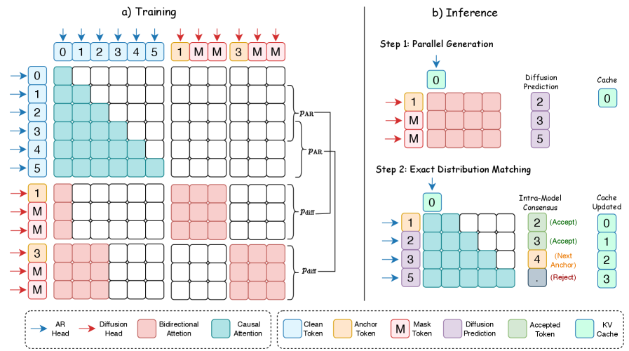
Training therefore reduces to a masked-denoising objective on the diffusion projections only: corrupt a block to (anchor, masks), supervise the diffusion head to reconstruct the true tokens given the AR KV. Because the AR head and its KV define the target distribution explicitly, no separate noise schedule on the backbone is needed.
Results
The authors evaluate on Qwen3-1.7B/4B/8B with the AR backbone frozen across all sizes. On MATH-500 with Qwen3-8B, Orthrus achieves a 6× throughput speedup over the AR baseline at strictly lossless accuracy — i.e., the consensus mechanism reproduces the AR sample distribution exactly — while Fast-dLLM-v2 at comparable speedups suffers substantial accuracy degradation. The paper’s headline figure of 7.8× corresponds to the most favorable configuration.
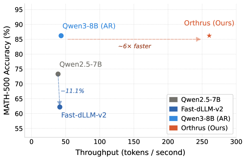
The block-size ablation isolates where the speedup comes from. Because the entire K-block is processed in a single forward pass against a pre-existing KV cache, per-pass latency is essentially flat in K. Scaling from K=4 to K=32 raises tokens-per-forward (TPF) to 6.35 and yields a 3.6× throughput multiplier with no latency penalty, motivating K=32 as the default. Note that TPF < K is expected: the consensus check rejects some parallel proposals, so realized acceptance is roughly 6.35/32 \approx 0.20 at K=32 — meaning gains come from cheap parallel proposals plus a non-trivial accept rate, not from accepting all K.
Limitations and open questions
- The “lossless” claim hinges on the AR consensus check; the paper’s quantitative speedups are net of rejections on MATH-500, but acceptance rates on long-form, less-structured generation (dialogue, code with high entropy) are not reported and are likely lower.
- Only Qwen3 is evaluated. Whether the 16% trainable-parameter diffusion head suffices for models with different attention patterns (GQA ratios, sliding-window, MoE routing) is untested.
- The diffusion head still adds per-layer compute and a second set of projections; on memory-bandwidth-bound hardware the wins are real, but on compute-bound regimes (small batch, short context) the picture may invert.
- No analysis of how acceptance scales with K beyond 32, nor of interaction with speculative decoding, which is structurally similar (draft + verify).
Why this matters
Orthrus reframes parallel decoding as a frozen-backbone adapter problem rather than a new pretraining regime: by routing a trainable diffusion head through the AR model’s own KV cache and verifying against the AR head, it gets diffusion-style block parallelism with AR-exact outputs and no extra historical KV memory. If the acceptance rates hold up outside math benchmarks, this is a cleaner drop-in than speculative decoding because the “draft” model is the target model.
Source: https://arxiv.org/abs/2605.12825
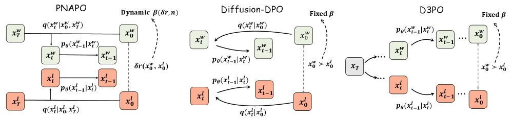
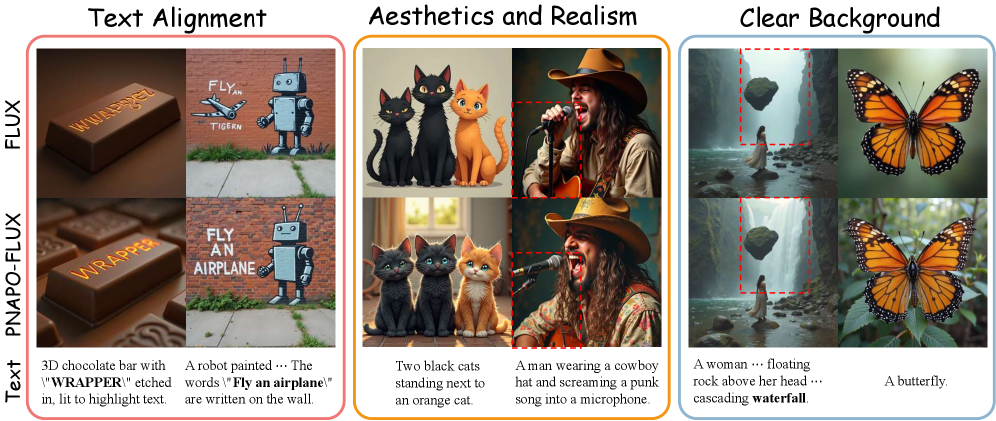
Offline Preference Optimization for Rectified Flow with Noise-Tracked Pairs
Problem
DPO-style alignment for diffusion models has a structural mismatch with rectified flow (RF). Standard preference datasets store only (c, \boldsymbol{x}_0^w, \boldsymbol{x}_0^l) — prompt, winner, loser. To compute a DPO loss for diffusion, one needs intermediate latents \boldsymbol{x}_t along the reverse trajectory, and Diffusion-DPO obtains them by sampling fresh forward noise \boldsymbol{x}_t = \alpha_t \boldsymbol{x}_0 + \sigma_t \boldsymbol{\epsilon} with \boldsymbol{\epsilon} \sim \mathcal{N}(0, I). For RF, this is doubly wrong: (i) RF trajectories are nearly straight lines indexed by a specific prior \boldsymbol{x}_T, so an independently drawn \boldsymbol{\epsilon} no longer corresponds to the actual generative path; (ii) the variance from this mismatch inflates gradient noise and slows convergence. Alternatives like D3PO recover trajectories by running the reverse process iteratively, which is expensive.
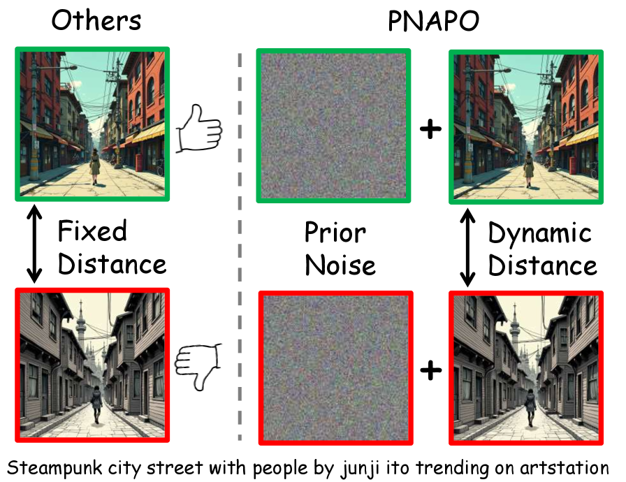
Method: PNAPO
The fix is conceptually simple — store the prior noise that produced each image — but it changes the data schema and the surrogate. PNAPO replaces the standard triplet with a sextuple (c, \boldsymbol{x}_T^w, \boldsymbol{x}_0^w, \boldsymbol{x}_T^l, \boldsymbol{x}_0^l, \delta r).
Off-policy data construction. Prompts come from DiffusionDB, filtered by Detoxify, deduplicated by Jaccard and CLIP cosine (>0.8), and rebalanced via 100-cluster KNN resampling, yielding 20k prompts. For each prompt the current RF model generates two images from independently sampled priors \boldsymbol{x}_T^w, \boldsymbol{x}_T^l \sim \mathcal{N}(0,I) using Euler discrete sampling (50 steps, guidance 1). HPSv2.1 supplies a continuous reward gap
\delta r = r_\theta(\boldsymbol{x}_0^w) - r_\theta(\boldsymbol{x}_0^l),
which both labels winner/loser and grades the magnitude of the preference.
RF-consistent surrogate via straight-line interpolation. Because RF transports \boldsymbol{x}_T to \boldsymbol{x}_0 along an approximately straight path, intermediate states are estimated by linear interpolation rather than re-noising:
\boldsymbol{x}_t = (1-t)\,\boldsymbol{x}_0 + t\,\boldsymbol{x}_T,\quad t \in [0,1].
This pins the trajectory to the actual prior used at generation time, eliminating the variance of resampling \boldsymbol{\epsilon} and giving a tighter surrogate for the DPO objective. Figure 3 contrasts this with Diffusion-DPO’s stochastic forward noising and D3PO’s iterative reverse rollouts.
Dynamic regularization. Standard DPO uses a fixed \beta controlling KL to the reference. PNAPO modulates the regularization based on (i) the reward gap \delta r and (ii) training step n: pairs with larger \delta r — clearer preferences — are pushed harder; the schedule is annealed across n to stabilize late training. The intuition is that small-margin pairs are noisy proxies and should not be allowed to drag the policy as aggressively as high-margin ones.
The resulting framework is RL-free and offline: data is generated once from the reference RF policy and reused for gradient updates against an interpolation-based DPO loss with adaptive \beta.
Results
Experiments use FLUX.1-dev and SD3-Medium, with AdamW at 1\text{e-}6 on 8 H800s; \beta = 2000 (FLUX uses 5000 — note table reports inverse mapping for the two models). Evaluation uses HPDv2 (3200 prompts) and OPDv1 (7459 prompts), scored by PickScore, HPSv2.1, ImageReward, LAION Aesthetic, and CLIP, plus GenEval.
On FLUX/HPDv2, PNAPO reaches HPSv2.1 31.71 vs DPO 30.84 and base FLUX 30.50; ImageReward 1.217 vs DPO 1.185; Aesthetic 6.475 vs 6.307. On FLUX/OPDv1: HPSv2.1 32.10 vs 30.79 (DPO), Aesthetic 6.692 vs 6.548, CLIP 36.89 vs 36.19. SD3-M shows the same ordering — e.g., HPDv2 HPSv2.1 31.62 (PNAPO) vs 31.13 (DPO) vs 30.83 (SFT). Win-rates of baselines against PNAPO are below 50% on essentially all metrics on both models (SFT-FLUX HPSv2.1 reports 88.4%, but this is win-rate of PNAPO against SFT given the table’s caption convention; numerically PNAPO scores higher).
The efficiency story is the more striking one. Reported training cost on H800:
- DPO-SD3 ~249.6 GPU-h vs PNAPO-SD3 ~20.8 GPU-h (≈12×).
- DPO-FLUX ~422.4 GPU-h vs PNAPO-FLUX ~35.2 GPU-h (≈12×).
The order-of-magnitude reduction is consistent with the variance argument: with the trajectory pinned to the true prior, far fewer gradient steps are needed for the policy to move on the reward.
Limitations and open questions
- The straight-line interpolation is exact only for an idealized rectified flow; trained RF models retain residual curvature, so the surrogate is biased, just less so than independent forward noising. The paper does not quantify this bias.
- Reward signal is HPSv2.1 alone, both for labeling and (in part) for evaluation, which risks reward hacking and reward-model overfitting; cross-reward ablations are not reported.
- The dynamic-\beta schedule is described in terms of \delta r and step n but the exact functional form is not in the included sections; sensitivity to its shape is unclear.
- All gains are on T2I RF models; whether prior-noise tracking helps DDPM-family models (where trajectories are not straight) is open.
- Off-policy data is generated from the model itself; iterative self-improvement could compound reward-model biases over rounds.
Why this matters
Rectified flow’s defining property — straight, prior-indexed trajectories — was being thrown away by preference pipelines inherited from diffusion. Storing the prior noise alongside winner/loser images and using \boldsymbol{x}_t = (1-t)\boldsymbol{x}_0 + t\boldsymbol{x}_T is a small data-schema change that yields ~12× lower training cost and consistent reward-model gains, suggesting RF alignment should be redesigned around trajectory identity rather than retrofitted from DDPM-DPO.
Source: https://arxiv.org/abs/2605.09433
Revisiting DAgger in the Era of LLM-Agents
Long-horizon LM agents face a familiar imitation-learning pathology: a single early action error shifts the state distribution off the teacher’s manifold, and subsequent decisions are made from contexts the student never saw during training. The paper frames the post-training landscape as a tradeoff between two failure modes. Supervised fine-tuning (SFT) on teacher trajectories provides dense per-token supervision but is purely off-policy with respect to the student, so it inherits classical covariate shift bounds (regret quadratic in horizon). RL with verifiable rewards (e.g., GRPO) is on-policy and avoids that mismatch but supplies only a terminal R(\tau,x)\in\{0,1\}, which is weak signal across trajectories that can span dozens of tool calls. The authors revisit Dataset Aggregation (DAgger) as the natural synthesis: rollouts are generated under a state distribution induced by the student, while labels come from the stronger teacher.
Setup and algorithm
The multi-turn agent is modeled with state s_t \triangleq (x, a_{1:t-1}, o_{1:t-1}) accumulating prompt, prior actions, and environment observations. At each turn, a_t \sim \pi(\cdot\mid s_t) and o_t \sim \mathrm{Env}(\cdot\mid x, a_{1:t}, o_{1:t-1}), terminating on a finish action or at T_{\max}. A verifier returns R(\tau,x)\in\{0,1\} — for SWE-Gym, whether the produced patch passes the held-out unit tests.
DAgger here operates at turn-level interpolation rather than token-level. Each rollout step samples the acting policy from a mixture \pi_{\mathrm{behave}}(\cdot\mid s_t) = \beta\,\pi_e(\cdot\mid s_t) + (1-\beta)\,\pi_\theta(\cdot\mid s_t), i.e., with probability \beta the teacher emits the turn, otherwise the student does. After the trajectory unrolls, the teacher \pi_e is queried on every visited state s_t to produce a target action a_t^\star \sim \pi_e(\cdot\mid s_t), and the student is updated by the standard SFT loss \mathcal{L}(\theta) = -\mathbb{E}_{s_t \sim d^{\pi_{\mathrm{behave}}}}\big[\log \pi_\theta(a_t^\star \mid s_t)\big]. Two properties follow. First, as \beta \to 0, the state distribution d^{\pi_{\mathrm{behave}}} approaches the deployment-time distribution d^{\pi_\theta}, so the student is trained on the contexts it actually encounters — directly attacking covariate shift. Second, supervision remains dense: every turn yields a teacher action label rather than a single terminal scalar.
The student is Qwen3-4B-Instruct-2507 or Qwen3-8B; the teacher is the larger Qwen3-Coder-30B-A3B-Instruct. Training uses 2,338 SWE-Gym tasks; evaluation uses a 100-instance SWE-Gym Holdout (in-domain) and 466 of the 500 SWE-Bench Verified tasks (34 Matplotlib instances fail to build in their Docker environment; the authors report <1% aggregate impact from this exclusion).
Empirical findings
The four research questions structure the experiments: aggregate effectiveness vs. SFT / GRPO / on-policy distillation, training stability under matched compute, direct measurement of covariate shift, and qualitative behavioral changes. The covariate-shift diagnostic is the most mechanistically informative: the authors measure token-level reverse KL D_{\mathrm{KL}}(\pi_\theta \| \pi_e) evaluated on contexts visited by the student itself.
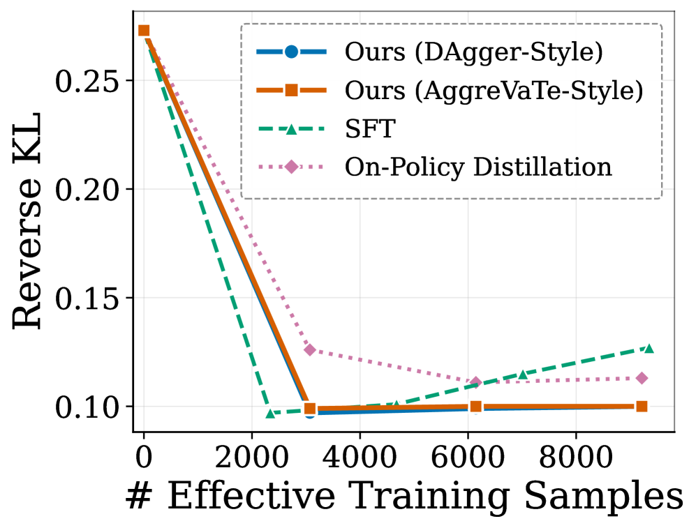
The relevant comparison is between SFT and DAgger on the student’s own state distribution. SFT minimizes D_{\mathrm{KL}} on teacher-visited states by construction, but those are not the states encountered at deployment; the figure shows that on student-visited contexts, the SFT model’s divergence from the teacher remains substantially higher than the DAgger-trained student, which is explicitly trained to imitate the teacher under d^{\pi_\theta}. This is the empirical signature of covariate shift: SFT’s training distribution and evaluation distribution disagree, and the disagreement compounds across turns.
Limitations and open questions
Several points warrant scrutiny. (1) DAgger requires online teacher queries on every student-visited state, which for a 30B-parameter teacher across multi-turn SWE-Gym rollouts is expensive — the matched-compute comparison with GRPO is therefore the load-bearing experiment, and details of how compute is normalized (teacher inference vs. student gradient steps) determine how the result generalizes. (2) The mixing schedule \beta is a free hyperparameter; classical DAgger anneals \beta_t \to 0, but the optimal schedule for LM agents with stochastic, high-branching action spaces is not characterized. (3) Teacher labels are themselves stochastic samples, not optimal actions; if the teacher is wrong on out-of-distribution student states (which DAgger deliberately produces), the student inherits those errors with no verifier-based correction. A hybrid with verifiable-reward filtering on teacher labels is an obvious next step. (4) Results are confined to SWE-Gym / SWE-Bench Verified with one teacher–student family; whether the gains transfer to web agents, tool-use benchmarks, or settings without an executable verifier is open.
Why this matters
DAgger gives a principled answer to the dense-supervision-vs-on-policy-state-distribution dilemma that currently splits LM-agent post-training into SFT and RLVR camps. Reframing it for turn-level mixing of a strong teacher with a student policy is a small algorithmic change with a clean theoretical justification, and the reverse-KL diagnostic on student-visited contexts is a useful, transferable instrument for detecting covariate shift in any multi-turn agent pipeline.
Source: https://arxiv.org/abs/2605.12913
Hacker News Signals
When “idle” isn’t idle: how a Linux kernel optimization became a QUIC bug
Cloudflare’s post-mortem on a QUIC connection death spiral traces the root cause to SO_TIMESTAMPING interactions with the Linux kernel’s receive-buffer coalescing path. When a UDP socket is idle — no packets arriving — the kernel’s GRO (Generic Receive Offload) layer can hold partially-assembled segments in a per-CPU cache rather than flushing them immediately. The assumption is that more packets will arrive and can be coalesced, reducing per-packet overhead. Under QUIC, however, this interacts badly with the loss-detection and congestion-control timers: if the kernel delays delivering an ACK-eliciting packet long enough, the sender’s PTO (probe timeout) fires, retransmitting. The retransmit then triggers further coalescing delay, and the connection spirals into repeated PTO-driven retransmissions at minimum congestion window — effectively stalling throughput while keeping the connection technically alive.
The fix required explicitly flushing the GRO cache by setting SO_BUSY_POLL or using epoll with EPOLLEXCLUSIVE in a way that forces kernel-side flush on each event loop iteration. The post walks through the udp_gro_receive call path and explains why the per-CPU napi cache doesn’t get flushed unless either (a) the GRO timer fires, (b) another packet arrives on the same flow, or (c) the application explicitly drains via a busy-poll hint.
The deeper issue is that GRO was designed around TCP semantics where the kernel owns both sides of the coalescing decision. QUIC running over UDP forces the application to implement its own reliability, so kernel-level batching optimizations that are transparent to TCP become observable and hazardous at the QUIC layer. The post quantifies the impact: affected connections could sit in the death spiral for tens of seconds before either recovering or timing out at the QUIC idle-timeout boundary.
Microsoft BitLocker – YellowKey zero-day exploit
The YellowKey disclosure demonstrates that BitLocker’s pre-boot authentication can be bypassed by placing specific files on a USB drive that is present during boot. The technical claim is that the Windows Boot Manager, when it enumerates removable media for BCD (Boot Configuration Data) entries, can be made to load an attacker-supplied BCD that redirects execution or disables integrity checks before the TPM unseals the VMK (Volume Master Key).
The critical detail is that this does not require physical modification of the target drive or any decapping of the TPM. The attack surface is the BCD parsing code in bootmgr.efi, which, under certain configurations, processes BCD stores from removable media without requiring them to be signed by a trusted key. If Secure Boot enforcement is incomplete — specifically if the DBX (forbidden signature database) is not updated or if a signed-but-vulnerable bootloader is still trusted — an attacker with physical access for the duration of one boot cycle can extract the VMK.
This falls into a category of attacks previously explored by researchers at Dolos Group and others: the TPM-only BitLocker configuration (no PIN, no USB key) relies entirely on the chain from UEFI Secure Boot through the boot manager to establish PCR measurements that gate TPM unsealing. Any signed component in that chain that can be coerced into misreporting PCR values, or any BCD processing path that runs before PCR measurement is finalized, breaks the security model.
The practical mitigation is BitLocker with a pre-boot PIN plus an updated Secure Boot DBX that distrusts the vulnerable bootloader binaries. TPM-only configurations on domain-joined machines remain exposed until Microsoft ships a patched bootmgr. The “backdoor” framing in the press is imprecise; this is more accurately a logic flaw in BCD source enumeration during pre-OS boot.
Interfaze: A new model architecture built for high accuracy at scale
The Interfaze blog post describes an architecture they call a “hierarchical mixture of experts with dynamic context routing,” though the implementation details are thin. The stated claim is that the model achieves higher accuracy per parameter than transformer-dense baselines by routing not just tokens but entire context segments to specialized sub-networks, with routing decisions conditioned on a compressed summary of the full sequence rather than only the current token.
The architectural idea — routing at the segment or document level rather than per-token — addresses a known weakness of standard sparse MoE: token-level routing ignores long-range dependencies in the gating decision, so topically coherent content can be split across unrelated experts. By computing a global context embedding (apparently via a small attention-based summarizer) and conditioning the router on it, the claim is that expert utilization becomes more semantically coherent.
The post provides benchmark numbers on a handful of reasoning and coding tasks where they assert outperformance over GPT-4o and Claude 3.5 Sonnet on specific subsets, but the evaluation methodology is not fully disclosed — no details on prompt construction, sampling parameters, or whether the comparisons are cherry-picked tasks. There is no paper, no model weights, and no reproducible artifact linked.
The HN discussion is appropriately skeptical: the architecture description is vague enough that it is difficult to distinguish genuine novelty from marketing copy. The segment-level routing idea has precedent in work like Longformer’s global attention tokens and hierarchical transformers, and the claim that this constitutes a fundamentally new architecture requires more rigorous ablation than a blog post provides. Treat as a product announcement with speculative technical framing until a preprint or independent evaluation appears.
Source: https://interfaze.ai/blog/interfaze-a-new-model-architecture-built-for-high-accuracy-at-scale
Show HN: Statewright – Visual state machines that make AI agents reliable
Statewright is a library that lets developers define agent control flow as explicit finite-state machines (FSMs) with typed transitions, then execute those FSMs as the scaffolding around LLM calls. The value proposition is engineering-level: FSMs provide a formal model where every reachable state is enumerable at definition time, which makes it possible to audit, test, and constrain agent behavior in ways that are difficult with purely prompt-driven or chain-of-thought agents.
The implementation uses a visual editor that exports to a JSON or YAML state graph. At runtime, each state can have an associated LLM call, tool invocation, or deterministic handler. Transitions are guards evaluated either deterministically (structured output parsing) or via a small classification call. The key constraint is that the agent cannot transition to a state not declared in the graph — there is no freeform “next action” decision; the LLM’s role is to populate parameters for the current state and signal which defined transition to follow.
This is essentially the approach advocated in the “language agents as Markov decision processes” framing, but implemented as a developer tool rather than a research artifact. The practical benefit for production agents is that you get an explicit audit log that maps to named states rather than an opaque sequence of token completions, and you can write deterministic unit tests against the transition graph by mocking LLM responses.
The limitation is expressiveness: tasks requiring genuinely open-ended planning — where the set of required states cannot be enumerated in advance — do not fit naturally into a fixed FSM. The library addresses this partially with “dynamic state expansion,” but the mechanism is not fully documented. For well-scoped workflow automation (form filling, multi-step API orchestration, customer service routing), this is a reasonable engineering choice over unstructured agent loops.
Cost of enum-to-string: C++26 reflection vs. the old ways
Vittorio Romeo’s benchmark post examines the runtime and compile-time cost of converting enum values to their string names using four approaches: a hand-written switch statement, a macro-generated lookup table (X-macros), a third-party library (magic_enum, which uses compiler-specific __PRETTY_FUNCTION__ / std::source_location hacks to extract enum names at compile time via template instantiation), and the upcoming C++26 static reflection via std::meta.
The performance story is largely compile-time dominated. magic_enum is notorious for exploding template instantiation counts: for an enum with N enumerators, it instantiates O(N) function templates during name extraction, which hits compile-time limits at around N=128 by default and produces noticeably slower builds for large enums. The X-macro approach has zero compile-time overhead beyond string literal concatenation but requires invasive macro discipline at the definition site.
C++26 reflection with std::meta::enumerators_of provides a clean solution: the compiler exposes the enum’s enumerators as a compile-time range of std::meta::info values, from which names can be extracted via std::meta::identifier_of. This allows a straightforward constexpr array construction without template explosion:
constexpr auto names = []<auto... Es>(std::integer_sequence<std::size_t, Es...>) {
    return std::array{std::meta::identifier_of(Es)...};
}(/* enumerator pack from std::meta::enumerators_of */);
Romeo’s benchmarks show that the reflection-based approach matches the switch statement at runtime (both compile to a bounds-checked array lookup), eliminates the N-template instantiation problem, and produces cleaner, definition-site-independent code. The main limitation is toolchain availability: C++26 reflection requires recent Clang with -freflection or EDG-based compilers; no GCC support yet.
Source: https://vittorioromeo.com/index/blog/refl_enum_to_string.html
Linux gaming is faster because Windows APIs are becoming Linux kernel features
The article covers two distinct kernel developments that reduce the overhead of running Windows games under Proton/Wine: the FUTEX_WAITV syscall (merged in 5.16) and the more recent work on NT synchronization primitives (ntsync) that landed in 6.14.
FUTEX_WAITV allows a thread to wait on a vector of futexes simultaneously, which maps directly onto WaitForMultipleObjects semantics. Previously, Wine implemented WaitForMultipleObjects by creating a dedicated kernel thread per waitable object and using signals or eventfd to aggregate wakeups — significant overhead for games that wait on dozens of synchronization objects per frame.
ntsync goes further: it implements the full NT kernel object model (mutexes, events, semaphores with NT semantics) as a character device with ioctls. The key NT semantic that POSIX primitives cannot express directly is that NT mutexes are owned and recursive, NT events have both auto-reset and manual-reset modes with specific pulse semantics, and WaitForMultipleObjects with WAIT_ALL must atomically acquire all objects or none. ntsync implements these in kernel space as a ntsync_device with per-object state tracked in kernel memory, allowing Wine to issue a single NTSYNC_IOC_WAIT_ANY or NTSYNC_IOC_WAIT_ALL ioctl instead of the previous userspace emulation path.
Benchmark numbers from the article and associated Phoronix testing show measurable frame-time variance reductions in synchronization-heavy titles — games using many short-lived mutex acquisitions per frame show the largest gains, with some titles reporting 10-20% throughput improvements. The broader implication is that Proton’s compatibility ceiling is increasingly determined by GPU drivers and Direct3D translation quality rather than synchronization overhead.
Rewrite Bun in Rust has been merged
PR #30412 merges a rewrite of Bun’s HTTP server internals from Zig to Rust, specifically the bun.http module that handles the server-side request/response lifecycle. This is notable because Bun has been a high-profile Zig project, and the move to Rust for a performance-critical subsystem signals a pragmatic rather than ideological stance on language choice.
The technical justification in the PR discussion centers on Rust’s tokio ecosystem and the maturity of async HTTP libraries (hyper, h2) versus the state of Zig’s async I/O story. Zig’s async/await was removed from the language in 0.12 pending a redesign, leaving projects that need structured async concurrency to either implement their own runtime or use synchronous threading models. Bun’s existing Zig HTTP server used a custom event-loop integration; the Rust rewrite can leverage tokio’s battle-tested executor and hyper’s HTTP/1.1 and HTTP/2 implementations directly.
The interop boundary is handled through a C FFI layer: Zig calls into the Rust HTTP server via extern "C" functions, and the Rust side calls back into Zig for JavaScript execution via the same mechanism. The PR adds a build.rs that compiles the Rust crate as a static library linked into the final Bun binary.
The HN discussion raises the obvious question of whether this signals broader Zig-to-Rust migration in the codebase. The Bun team’s response is that the rewrite is scoped to the HTTP server and motivated by specific library availability, not a general language switch. The more interesting engineering question is whether the FFI boundary introduces measurable overhead on the hot path; the PR does not include before/after benchmarks, which is a notable omission for a performance-motivated rewrite.
Show HN: A modern Music Player Daemon based on Rockbox firmware
rockbox-zig reimplements the Rockbox audio firmware’s playback engine as a networked music daemon, with the core DSP and codec layer ported to Zig and a gRPC API replacing the traditional MPD protocol. Rockbox’s codec library supports a wide range of lossless and lossy formats (FLAC, APE, Musepack, Speex, AAC, WavPack) with fixed-point DSP tuned for embedded targets; porting it to Zig preserves that codec breadth while making the binary deployable on standard Linux servers and desktop systems.
The gRPC interface is a deliberate departure from the original MPD text protocol. The .proto definitions expose playback control, queue management, and metadata queries as typed RPC calls, which makes building clients in any gRPC-supported language straightforward without implementing a line-oriented text parser. The project includes a web UI client and a CLI.
The Zig port of the Rockbox C codec code is largely a mechanical translation — Zig’s C interop allows calling the original Rockbox C directly via @cImport, so much of the codec layer is the original C compiled under the Zig build system rather than a true rewrite. The Zig-native parts are the daemon infrastructure: event loop, gRPC server (using a Zig gRPC library), and audio output via ALSA/PulseAudio/PipeWire backends.
The interesting technical aspect is using Rockbox’s fixed-point DSP on a platform with FPU. Rockbox’s DSP was designed to avoid floating point for ARM7/ColdFire targets; on x86-64, the fixed-point paths will be slower than equivalent floating-point DSP, though for audio playback the difference is irrelevant. The project is in early development; the queue and playlist state management is not yet persistent across restarts.
Noteworthy New Repositories
samchon/ttsc
ttsc is a drop-in TypeScript compiler wrapper that exposes a plugin API layered on top of typescript-go (the official Go-rewrite of tsc). The key value proposition is twofold: (1) compiler-powered transform plugins that run inside the type-checker’s own pass rather than as a post-processing step, enabling transforms that have access to full type information without a separate ts-morph traversal; and (2) integration of a TypeScript linter (analogous to ts-eslint rules) directly into the compile pipeline, claiming ~20x throughput improvement over running ESLint separately. Because the underlying compiler is written in Go and compiled to a native binary, the cold-start and incremental-rebuild costs are substantially lower than the Node.js tsc. Plugin authors implement a typed interface and register hooks at well-defined compiler phases. Type-safe execution refers to the guarantee that plugin-generated or plugin-transformed code is re-checked by the same type system pass, not emitted blindly. This is relevant for codegen use cases (e.g., DTO validators, ORM schema derivation) where existing solutions like ttypescript or ts-patch patch the Node.js compiler internals and can break across tsc versions. Worth watching for teams that maintain non-trivial TypeScript transform pipelines or run lint at scale in CI.
Source: https://github.com/samchon/ttsc
xataio/xata
Xata is an open-source, cloud-native Postgres platform centered on two non-standard primitives: copy-on-write database branching and scale-to-zero compute. Branching uses a CoW storage layer so that creating a branch from a multi-gigabyte database is instantaneous and storage overhead is proportional only to diverging writes, not to the full dataset size. This is the same semantic model as Neon’s branching, implemented here as a fully open-sourced stack. Scale-to-zero suspends compute when idle and resumes on connection, targeting serverless and preview-environment workloads where cost-per-active-hour matters. The platform exposes standard Postgres wire protocol, so existing drivers and ORMs require no changes. Under the hood, the architecture separates storage from compute — a common pattern in cloud-native databases (Aurora, Neon, AlloyDB) — but the open-source release means operators can self-host the full stack rather than being locked to a managed service. The 835-star traction shortly after open-sourcing suggests demand for a self-hostable Neon alternative. Relevant to teams building ephemeral per-PR database environments, staging pipelines, or multi-tenant SaaS where tenant isolation via branching is architecturally cleaner than schema-per-tenant.
Source: https://github.com/xataio/xata
bkywksj/knowledge-base
A local-first personal knowledge base desktop application built on Tauri 2.x (Rust backend), React 19 (frontend), and SQLite as the single storage substrate. Full-text search uses SQLite’s FTS5 extension, keeping search entirely in-process with no external search daemon. Bidirectional linking and a knowledge graph are implemented on top of a standard link-extraction pass over Markdown AST, with graph edges stored in SQLite. Sync is designed around note-level granularity rather than full-database sync: the scheduler performs incremental, bidirectional reconciliation over WebDAV, S3, or filesystem sync providers, with a whole-library ZIP backup fallback. The AI layer supports OpenAI-compatible endpoints, Ollama, and arbitrary custom providers via a tool-calling framework — meaning the agent can invoke defined tools (search, create note, link notes) rather than just generating text. Encryption is implemented as a vault abstraction with per-vault keys and a PIN-gated hidden-notes feature. Import handles .md, .txt, .pdf, and .docx with automatic charset sniffing. The Tauri + Rust choice gives a small binary footprint and no Electron-style Chromium bundling overhead. Zero cloud dependency is a genuine architectural property, not a marketing claim — all data paths terminate locally.
Source: https://github.com/bkywksj/knowledge-base
mvm-sh/mvm
mvm is a bytecode interpreter and virtual machine targeting Go source code, with stated ambitions beyond Go. The “fast interpreter” framing suggests it compiles Go to an internal bytecode IR and executes that rather than invoking go build and running native code, which enables use cases like scripting, plugin sandboxing, and REPL-style execution without the full toolchain compile latency. This is the same design space as yaegi (Traefik’s Go interpreter) and gopherlua for Lua-in-Go, but positioned as a general VM rather than an embedding-first tool. The “and beyond” language support hint suggests either a common bytecode target for multiple frontend languages or planned language extensions via a custom grammar. Key technical questions — register-based vs. stack-based VM, GC strategy, FFI for calling into native Go packages, and whether the type system is enforced at bytecode level — are not fully documented yet but are the axes on which this will compete with yaegi. Relevant for plugin architectures in Go services where dynamic code loading without cgo or os/exec is desirable, and for build-system acceleration in monorepos where full recompilation on every test run is the bottleneck.
Source: https://github.com/mvm-sh/mvm
awizemann/harness
Harness is an LLM-driven automated UI testing tool for iOS Simulator, macOS native apps, and web apps. The operator writes a plain-language goal (e.g., “log in and create a new project”); an agent loop translates the goal into UI actions, executes them via accessibility APIs or WebDriver, observes the resulting state, and continues until goal completion or failure. The output is a friction report — where the agent got stuck, retried, or failed — rather than a pass/fail assertion. This is closer to exploratory testing than traditional scripted UI automation (XCTest, Playwright). The technical stack is Swift 6 on macOS 14+, which means it can use the modern Swift concurrency model (async/await, structured concurrency) for the agent loop and native XCTest/Accessibility APIs for simulator interaction without a bridge layer. The LLM integration likely follows a vision-language model or accessibility-tree-as-context approach — using the app’s accessibility hierarchy as structured input to the model rather than raw screenshots, though both approaches are plausible. The value proposition is catching UX regressions that are hard to express as deterministic assertions but obvious to a user navigating the app — a complement to, not replacement for, unit and integration tests.
Source: https://github.com/awizemann/harness
openlake-project/openlake
OpenLake targets the GPU data-ingestion bottleneck: the problem where GPU compute sits idle waiting for training data to arrive from distributed storage. The “hyper efficient storage for GPU workloads” framing points to an object store or file system designed around the specific access patterns of deep learning pipelines — large sequential reads, high concurrency from many GPU workers, and minimal metadata overhead per file. The architecture likely involves: a custom storage format optimized for sequential scan rather than random access, prefetch-aware scheduling, and possibly RDMA or GPUDirect support to reduce CPU involvement in the data path. The “blazing fast speeds” claim needs to be evaluated against concrete benchmarks (samples/sec, bytes/sec at various batch sizes) against baselines like FUSE-mounted S3, NFS, or purpose-built alternatives like IBM Storage Scale or NVIDIA Magnum IO. This is the same problem space as WebDataset, MosaicML’s StreamingDataset, and Google’s tf.data service — but positioned as a storage layer rather than a dataset API. Relevant to ML infrastructure teams running large-scale pretraining where I/O throughput, not compute, is the limiting factor.
Source: https://github.com/openlake-project/openlake
esengine/DeepSeek-Reasonix
A terminal-based AI coding agent built specifically around DeepSeek models, with the primary engineering differentiator being prefix-cache stability. DeepSeek’s KV-cache prefix caching is most efficient when the prompt prefix is kept constant across turns; agents that prepend dynamic content (timestamps, turn counters, mutable context) to the system prompt break cache locality and incur full prefill cost on every request. Reasonix is engineered to keep the system prompt and tool definitions static so the cache hit rate stays high across a long session, making it practical to “leave it running” on a long agentic task without the cost-per-token blowing up. The architecture is a standard tool-calling agent loop (observe, plan, act via shell/file/code tools) but the prompt construction discipline is the core contribution. At 2053 stars, it has significant traction in the DeepSeek user community. Worth examining for teams self-hosting DeepSeek inference with a caching proxy (e.g., SGLang’s RadixAttention or vLLM’s prefix caching) where prompt engineering for cache locality is a first-class concern. The terminal interface keeps the operational footprint minimal relative to web-based alternatives like Continue or Cursor.
Source: https://github.com/esengine/DeepSeek-Reasonix
t8y2/dbx
dbx is a 15 MB cross-platform database GUI client supporting MySQL, PostgreSQL, SQLite, Redis, MongoDB, DuckDB, ClickHouse, SQL Server, and additional backends. The small binary size is the headline technical claim — for comparison, DBeaver’s installer is ~100 MB and TablePlus is similar. Achieving this likely involves a non-Electron build (probably a native UI toolkit or a minimal WebView wrapper without bundling a full Chromium) and careful dependency management. Supporting heterogeneous backends — relational (MySQL, Postgres, SQLite, SQL Server), columnar (DuckDB, ClickHouse), document (MongoDB), and key-value (Redis) — in a single client requires a driver abstraction layer that normalizes query execution, result schema, and metadata operations across fundamentally different wire protocols. The 1411-star count suggests genuine demand for a lightweight, portable alternative to heavier clients in the same space (DBeaver, TablePlus, DataGrip). Particularly relevant for developers who want a single tool across heterogeneous data stacks without a multi-hundred-MB install, or for environments where installing Electron-based tooling is restricted. The DuckDB and ClickHouse support is notable for analytics-heavy workflows where a GUI query tool saves iteration time over CLI.
Source: https://github.com/t8y2/dbx