Daily AI Digest — 2026-05-11
arXiv Highlights
Mean Mode Screaming: Mean–Variance Split Residuals for 1000-Layer Diffusion Transformers
Problem
Scaling DiTs to hundreds of layers exposes a failure mode that is invisible in standard loss curves until it is too late: a sudden, mean-dominated collapse in which token representations homogenize across the sequence and the network loses the centered variation that carries token-specific content. The authors call the trigger Mean Mode Screaming (MMS) and argue it is not a generic optimizer instability but a structural consequence of how residual writers interact with row-stochastic attention at depth. The practical stakes are that recipes which work at 30–60 layers (Post-Norm + RMSNorm, LayerScale, ReZero) silently fail or underperform at 400+ layers.
Geometry and the failure sequence
The analysis hinges on a token-axis split with J=\frac{1}{T}\mathbf{1}\mathbf{1}^\top and P=I-J, decomposing X = \mu(X) + c(X) = JX + PX. Two facts drive everything:
- Row-stochastic attention preserves the pure-mean component: A\mu(X)=\mu(X).
- The centered component is governed by c(AX)=PAPX, with contraction factor \mu_{\text{eff}}(A)\triangleq\|PAP\|_2.
Once \mu_{\text{eff}}<1 in deep layers, attention strictly contracts centered variation, and only residual branches can replenish it. If the residual updates themselves become mean-coherent, the network slides into a pure-mean fixed direction.
The right panel of Figure 2 shows \rho_T=\|\mu(X)\|_F/\|c(X)\|_F rising monotonically with depth across L0–L384, exactly the regime where the geometry predicts vulnerability.
Mechanism: alignment-amplification at residual writers
For any token-wise linear writer W (specifically W_O and FFN W_2), the gradient \nabla_W\mathcal{L}=\sum_t \delta_t y_t^\top admits an exact split into mean-coherent and centered pieces (cross-terms vanish under the sum):
\nabla_W\mathcal{L} = \underbrace{T\,\bar\delta\,\bar y^\top}_{\Delta W_\mu} + \underbrace{\sum_t \tilde\delta_t \tilde y_t^\top}_{\Delta W_c}.
The mean term is rank-1 and scales as \mathcal{O}(T) when \bar y, \bar\delta stop canceling; the centered term sums diffusively. Defining the alignment amplification
\mathcal{A}-1 = \frac{\sum_{s\neq t}(\delta_s^\top\delta_t)(y_s^\top y_t)}{\sum_t \|\delta_t\|^2\|y_t\|^2} \approx (T-1)\,\underbrace{\mathbb{E}_{s\neq t}[\cos(y_s,y_t)\cos(\delta_s,\delta_t)]}_{\kappa},
MMS is the transition \kappa: 0 \to \mathcal{O}(1) as forward and backward signals co-align across tokens. Once \kappa\to 1, the rank-1 mean mode hits its coherent \mathcal{O}(T) regime and shocks the writers. A second, compounding effect: as values homogenize across tokens, attention-logit gradients fall in the null space of the softmax Jacobian, so Q/K stop receiving useful signal — the network cannot self-correct via attention.
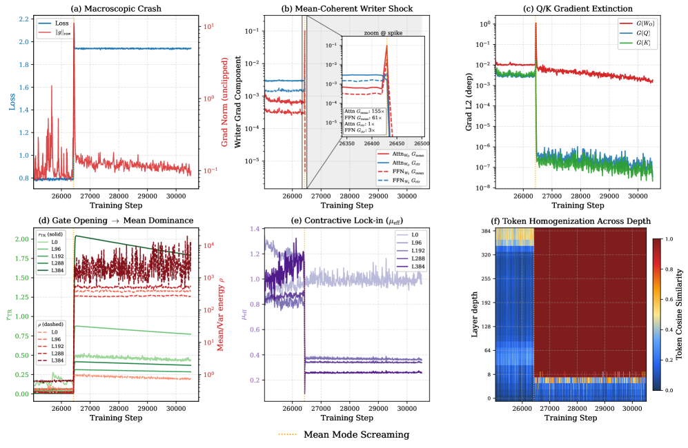
Figure 3 shows the trigger cleanly: the global gradient-norm spike is almost entirely in G_{\text{mean}}=\|\Delta W_\mu\|_F, while G_{\text{ctr}} shows no comparable amplification, and Q/K gradients are suppressed afterwards. Empirically at the spike step t^\star=3400 in the 400-layer run, active layers reach \mathcal{A}-1\approx 167, i.e., roughly 13\times writer-gradient amplification over the independent-token baseline, sitting on the absolute-coherence saturation envelope predicted by Eq. (6). The same near-saturation appears for both Attn_WO and FFN_W2, which rules out an attention-specific story and pins the failure to the writer interface.
Method: MV-Split residuals
The fix isolates and damps \Delta W_\mu without throttling \Delta W_c. Replace the Post-Norm merge with a subspace-routed residual using per-block, per-channel learnable gains \alpha,\beta\in\mathbb{R}^D:
Z_l = X_l + \beta\odot(PF_l) + \alpha\odot J(F_l - X_l), \qquad X_{l+1}=\text{RMSNorm}(Z_l).
Projecting before normalization decouples the two subspaces:
PZ_l = PX_l + \beta\odot(PF_l), \qquad JZ_l = (1-\alpha)\odot(JX_l) + \alpha\odot(JF_l).
The centered subspace is a standard residual stream with gain \beta; the mean subspace is a per-feature leaky integrator that contracts the trunk mean by 1-\alpha_d each layer. Crucially the backward pass inherits the same split:
\partial\mathcal{L}/\partial F_l = \beta\odot(PG_l) + \alpha\odot(JG_l),
so a small \alpha damps both the forward mean accumulation and the rank-1 \Delta W_\mu component while leaving centered branch-gradients at gain \beta. This is the structural distinction from LayerScale and ReZero, which apply a single residual gain and necessarily suppress \Delta W_\mu and \Delta W_c together. For the multimodal variant, J,P are applied segment-wise to avoid mixing image and text means in the residual control path.
Results
On a 400-layer single-stream DiT trained on ImageNet-2012 latents (frozen FLUX.2 VAE, Qwen3-0.6B text conditioning), MV-Split prevents the divergent collapse that crashes the un-stabilized Post-Norm baseline within the first 10k steps and tracks close to the baseline’s pre-crash trajectory while remaining substantially better than token-isotropic gating (LayerScale-style) controls. The same residual design scales to a 1000-layer run carried through ImageNet pretraining and post-training on a ~50k curated set, producing coherent text-to-image samples (Figure 1; weights at https://huggingface.co/StableKirito/mvsplit-dit-1000l).
Limitations and open questions
The headline experiments are validation rather than a competitive system: ImageNet-scale latents, a single backbone family, no FID/CLIP comparisons reported in the provided sections, and the 1000-layer run is a scale demonstration rather than a controlled ablation. The mechanism analysis is built on the equal-magnitude absolute-coherence proxy \hat\kappa, an upper envelope; tighter signed-coherence diagnostics would sharpen the predictive use of Eq. (6). The interaction between \alpha, \beta initialization and learning-rate/warmup schedules is deferred to appendices, and it is not yet clear whether MMS reappears under different normalization choices (e.g., QK-norm at extreme depth) or in autoregressive transformers where the same writer decomposition holds.
Why this matters
The paper gives an exact, falsifiable account of one specific instability that gates depth scaling in DiTs — rank-1 mean-coherent gradient accumulation at residual writers — and a minimal fix that targets that mode without damping the rest of the residual signal. If the alignment-amplification law generalizes, it provides a principled diagnostic (\hat\kappa, G_{\text{mean}}/G_{\text{ctr}}) and a design rule (decouple mean and centered residual gains) for any deep token-mixing architecture.
Source: https://arxiv.org/abs/2605.06169
Listwise Policy Optimization: Group-based RLVR as Target-Projection on the LLM Response Simplex
Problem
Group-based RLVR methods (GRPO, Dr.GRPO, DAPO, MaxRL, etc.) all sample K responses per prompt, compute a group-relative advantage, and update via a PPO-style surrogate. They differ mostly in how the advantage is normalized — by group std \sigma_G, by a constant, by group mean \mu_G — yet there is no unifying account of what distribution each is implicitly chasing, nor why the resulting first-order updates are stable. This paper recasts the entire family as a two-step target-projection procedure on a finite response simplex, and replaces the implicit first-order approximation with an explicit projection step.
Listwise distribution and the implicit target
For prompt x with K sampled responses \{y_k\}, define the listwise distribution
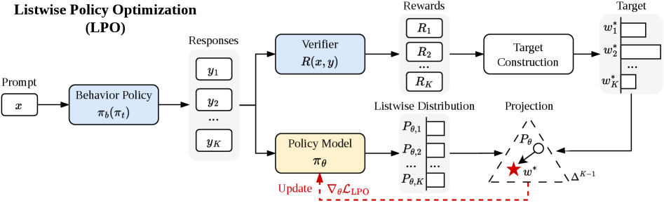
P_{\theta,k} = \mathrm{softmax}(s_\theta)_k, \quad s_{\theta,k} = \log\frac{\pi_\theta(y_k\mid x)}{\pi_b(y_k\mid x)},
which lives on \Delta^{K-1}. At the on-policy point \pi_\theta=\pi_b, P_\theta = \mathbf{1}/K. The authors define a local proximal RL objective on this simplex,
\max_{w\in\Delta^{K-1}} \hat J(w) = \sum_k w_k R_k - \tau D_{\mathrm{KL}}(w\,\|\,P_t),
with P_t the listwise distribution at the pre-update parameters. The unique maximizer is a Gibbs target
w^*_k = \mathrm{softmax}(\phi)_k,\quad \phi_k = R_k/\tau + s_{t,k}. \qquad (8)
On policy (P_t = \mathbf{1}/K), w^* = \mathrm{softmax}(R/\tau), and Proposition 1 shows that GRPO (\tau=\sigma_G), Dr.GRPO (\tau=1), and MaxRL (\tau=\mu_G) each recover this target as their implicit first-order linearization. Advantage normalization, in this view, is just an implicit choice of trust-region temperature.
LPO: explicit projection
Rather than the linearized PG step, LPO performs the two-stage update of Eq. (6):
- Target. Compute w^* in closed form via Eq. (8).
- Projection. Solve \theta' = \arg\min_\theta D(w^*\,\|\,P_\theta) for a chosen divergence D.

Two natural choices give two variants:
- \mathrm{LPO}_{\mathrm{fwd}}: forward KL D_{\mathrm{KL}}(w^*\,\|\,P_\theta) = -\sum_k w^*_k \log P_{\theta,k} + \text{const}, i.e. a weighted listwise cross-entropy over the K responses, mass-covering.
- \mathrm{LPO}_{\mathrm{rev}}: reverse KL D_{\mathrm{KL}}(P_\theta\,\|\,w^*), mode-seeking.
The projection gradients are bounded, zero-sum across the group (since both w^* and P_\theta are simplex-valued, gradients in s_\theta-space sum to zero), and self-correcting: as P_\theta\to w^*, the gradient vanishes. Theorem 2 gives a monotonic improvement bound: if the projection achieves \mathrm{TV}(P_{t+1}, w^*)\le\epsilon_{\mathrm{proj}} and |R_k|\le R_{\max},
\hat R(P_{t+1}) \ge \hat R(P_t) + \tau\bigl[D_{\mathrm{KL}}(w^*\|P_t) + D_{\mathrm{KL}}(P_t\|w^*)\bigr] - 2R_{\max}\epsilon_{\mathrm{proj}}.
The Jeffreys-divergence target gain is non-negative and strictly positive whenever w^*\ne P_t, in contrast to PG, which only guarantees descent on the linearized surrogate.
Implementation skeleton
For each prompt:
Sample K responses from pi_t; receive rewards R_k.
Compute s_{t,k} = log pi_t(y_k|x) - log pi_b(y_k|x).
phi_k = R_k / tau + s_{t,k}
w_star = softmax(phi)        # detached
For minibatch step over k:
    s_{theta,k} = log pi_theta(y_k|x) - log pi_b(y_k|x)
    P_theta = softmax(s_theta)
    loss = D(w_star, P_theta)   # forward or reverse KL
    backprop
The temperature \tau is matched to each baseline (\sigma_G, 1, \mu_G) so any gain is attributable to the projection, not to temperature tuning.
Results
LPO is evaluated on logic (Countdown-34/4), math (MATH → AIME24/25, AMC23, MATH500, Minerva, Olympiad), code (PRIME), and multi-modal geometry (Geometry3k), with backbones from 1.5B to 14B (Qwen3-1.7B/4B/8B/14B-Base, Qwen2.5-VL-3B-Instruct).
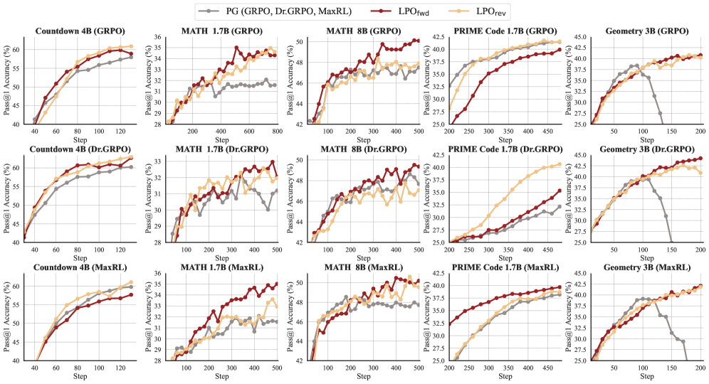
Across all three baseline temperature regimes and all four task domains, both \mathrm{LPO}_{\mathrm{fwd}} and \mathrm{LPO}_{\mathrm{rev}} dominate the matched PG baseline on Pass@1 throughout training. Because \tau is held identical to each PG counterpart, the curves isolate the effect of replacing the linearized PG step with the exact projection. The reverse-KL variant tends to be sharper (mode-seeking on w^*), while forward KL is more conservative; both inherit the bounded zero-sum gradients implied by simplex-valued projections.
Limitations and open questions
- The analysis is local-per-prompt; cross-prompt interactions and off-policy reuse beyond a single update step are not characterized.
- The response simplex has fixed K; the K\to\infty limit recovers the standard KL-regularized RL objective, but finite-K bias is not quantified.
- Only forward/reverse KL are evaluated; the framework admits any divergence (e.g., \alpha-divergences, \chi^2), and which divergence is optimal under what reward sparsity is unresolved.
- The improvement bound depends on \epsilon_{\mathrm{proj}}; in practice, this is controlled only implicitly through SGD step counts and learning rate.
- No reported numbers on absolute final accuracies relative to closed-source RLVR recipes (e.g., DAPO with full engineering); the comparison is apples-to-apples but narrow.
Why this matters
The paper supplies a clean geometric account of why advantage normalization choices in group-based RLVR behave like trust-region temperatures, and shows that the standard PG step is just a first-order linearization of an exact projection that admits a closed-form Gibbs target. Replacing the linearization with explicit divergence minimization gives monotonic-improvement guarantees and consistent empirical gains without retuning, which is a more principled lever than yet another advantage-normalization trick.
Source: https://arxiv.org/abs/2605.06139
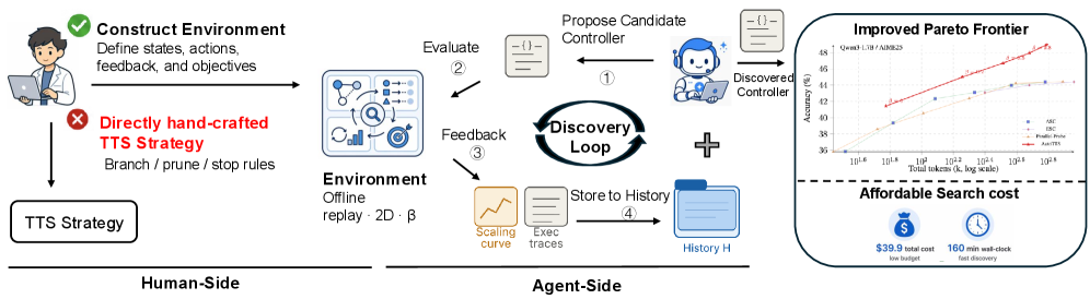
LLMs Improving LLMs: Agentic Discovery for Test-Time Scaling
Problem
Test-time scaling (TTS) — best-of-N, self-consistency, early stopping, adaptive branching, speculative pruning — is currently a cottage industry of hand-tuned heuristics. Each method picks a single slice of the width-depth allocation space and hand-codes thresholds. The authors argue that the design surface is large enough that human intuition leaves substantial Pareto improvements on the table, and that the right object for an LLM agent to optimize is not a single heuristic but an environment in which heuristics can be searched cheaply.
Formalism: width-depth control as a budgeted MDP
The paper casts adaptive inference as controller synthesis over a state s_t = (q, m_t, I_t, \ell_t, \Omega_t), where m_t is the number of branches instantiated, I_t \subseteq [m_t] is the active set, \ell_{t,i} is the depth (in fixed-length probe intervals of \Delta tokens) of branch i, and \Omega_t holds revealed probe answers (i, k, \omega_{i,k}). Cost accumulates as
\mathrm{Cost}(s_t) = \sum_{i=1}^{m_t} \ell_{t,i} + \kappa_{\mathrm{probe}} |\Omega_t|,
with admissible actions \{\texttt{BRANCH}, \texttt{CONTINUE}(i), \texttt{PROBE}(i), \texttt{PRUNE}(i), \texttt{ANSWER}\} subject to a global budget B. BRANCH opens a new chain and runs it for one interval; CONTINUE extends an active branch by \Delta tokens; PROBE reveals the current intermediate answer \omega_{i,\ell_{t,i}} without advancing the branch; PRUNE deactivates a branch but retains its history; ANSWER triggers aggregation.
This formulation subsumes existing methods as restricted policies on a 2D width-depth surface.
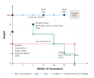
SC@64 sits at the maximum-width, full-depth corner; ASC and ESC adapt width at fixed full depth; Answer Consistency adapts depth on a single chain; ST-BoN expands wide then prunes. AutoTTS searches the full 2D space.
Method: AutoTTS
Three design choices make the search tractable:
Offline replay environment. For each (q, \text{model}) pair, N=128 trajectories are pre-sampled at temperature 0.7, each segmented into intervals of \Delta = 500 tokens. The branch prefixes z_{i,k} and probe signals \omega_{i,k} are precomputed and cached. A candidate controller’s decisions then index into this replay matrix — no LLM calls during discovery. Each controller is evaluated 64 times by subsampling from the pool of 128 to reduce variance.
Beta parameterization. Rather than letting the agent emit raw thresholds (which overfit to \mathcal{Q}_{\text{search}}), policies are parameterized through normalized \beta values. The agent writes code-defined controllers \pi(\cdot \mid s, \beta) where \beta governs branching, pruning, and stopping decisions in a way that transfers across budgets and models.
Execution trace feedback. Instead of returning only a scalar accuracy/cost to the explorer LLM, each evaluation returns a fine-grained trace of why the controller failed (e.g., pruned the eventually-correct branch at depth k, exhausted budget on a divergent chain, probed too rarely). This converts the agent’s task from black-box hyperparameter search into something closer to debugging.
The discovery loop uses Claude Code as the explorer LLM for five rounds. \mathcal{Q}_{\text{search}} is AIME24, and \mathcal{E}_{\text{search}} is the union of AIME24 environments across Qwen3-{0.6B, 1.7B, 4B, 8B}. The single controller maximizing accuracy on \mathcal{E}_{\text{search}} is fixed and transferred.
Results
The discovered controller is evaluated on held-out AIME25 and HMMT25 environments, which were never seen during discovery or model selection. The replay-based evaluation enables thousands of controller evaluations per round at the cost of a single offline trajectory pass; without it, the same search would require on the order of 64 \times |\mathcal{E}_{\text{search}}| live LLM rollouts per candidate. The held-out transfer to AIME25/HMMT25 across four model scales is the central empirical claim — the discovered controller, optimized only on AIME24, generalizes to new benchmarks and is reused across the 0.6B-8B Qwen3 range without per-model retuning.
Limitations and open questions
- The replay environment fixes the trajectory distribution at temperature 0.7 with \Delta = 500. Controllers that would benefit from temperature scheduling, variable interval lengths, or branch resampling cannot be expressed.
- N = 128 pre-sampled trajectories upper-bounds the achievable width; controllers requesting branch 129 have no replay data.
- Probe signals \omega_{i,k} are themselves LLM-generated intermediate answers and inherit the base model’s miscalibration — pruning decisions conditioned on \Omega_t propagate that bias.
- Discovery is restricted to AIME24; whether the same agent loop produces qualitatively different controllers when \mathcal{Q}_{\text{search}} is code or long-context QA is unaddressed.
- Five rounds of Claude Code is a small search budget; the search-vs-evaluation Pareto frontier is not characterized.
Why this matters
The contribution is methodological: by constructing an offline replay environment plus a parameterization that admits cheap, deterministic evaluation, the authors convert TTS algorithm design from a hand-crafted heuristic exercise into a search problem an LLM agent can run end-to-end. This is a concrete instance of the broader pattern where the bottleneck in LLM self-improvement is environment construction rather than the optimizer itself.
Source: https://arxiv.org/abs/2605.08083
Anisotropic Modality Align
Contrastive multimodal encoders (CLIP-style) are increasingly used as a “bridge” so that an MLLM can be trained on text-only data while expecting image embeddings at inference. This works only if text and image embeddings are interchangeable in the shared space. The persistent modality gap says they are not. This paper asks what the gap actually is geometrically, and finds that it is neither a global translation nor a generic distribution mismatch, but a low-rank anisotropic residual atop an already-shared dominant geometry.
The gap is not what you think
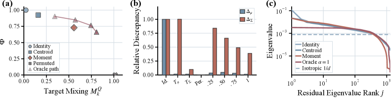
Using 1M paired image-text embeddings, the authors compare the centered covariances \Sigma_x and \Sigma_y. Two diagnostics matter. First, the spectral correlation C_\lambda = \mathrm{corr}(\log\lambda(\Sigma_x), \log\lambda(\Sigma_y)) = 0.845, i.e. the two modalities allocate variance across dominant directions in nearly the same way. Second, the principal-subspace overlap O_q = \tfrac{1}{q}\,\|(U_x^q)^\top U_y^q\|_F^2 sits well above the random baseline q/d: at q=128, O_{128}=0.441 versus q/d=0.100.
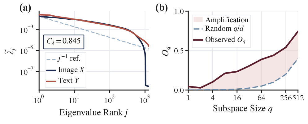
So the dominant directions are shared. What remains? After mean-centering, the residual cross-modal discrepancy is still large, its covariance spectrum deviates sharply from isotropy, and the energy is concentrated in a few directions. The reported anisotropy ratio is A_r=28.6 with effective dimension d_{\mathrm{eff}}/d = 0.284.
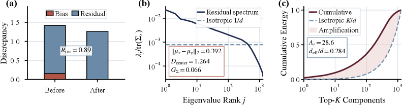
This reframes prior fixes: simple centroid shifts (e.g. C3) only chip away at a small isotropic-looking fraction, and aggressive target-replacement strategies destroy source semantic correspondence (Fig. 3). The right object to correct is the small anisotropic residual subspace.
AnisoAlign
The method fixes a shared frame instead of estimating modality-specific bases that may drift. Let \mu_t,\mu_i\in\mathbb{R}^d be empirical means and \Sigma_t,\Sigma_i the centered covariances. Define the joint structure matrix \Sigma = \Sigma_t + \Sigma_i + \lambda I, and let Q_U\in\mathbb{R}^{d\times r} contain its top-r eigenvectors. Then \mathbb{R}^d = U\oplus V with U=\mathrm{span}(Q_U), and any embedding decomposes as z_U = Q_U Q_U^\top z, \qquad z_V = z - z_U. \tag{1} U is the shared anisotropic subspace where the gap concentrates; V is the (near-isotropic) complement. All alignment operations are performed under this fixed decomposition: aggressive correction inside U to match the target distribution along the few anisotropic directions, and minimal modification in V to preserve the source’s semantic structure. This operationalises the principle the paper articulates — align with the target-modality distribution while preserving the semantic structure of the source modality — by separating the two objectives onto orthogonal subspaces rather than trading them off in a single global transform.
Empirical geometry
With LLM2CLIP-OpenAI-L-14-336 as encoder and Llama-3-8B-Instruct as LLM backbone, the authors compare Text (raw text embeddings), C3, ReAlign, and AnisoAlign on 10K paired samples, using images as target.
- Centroid discrepancy \Delta_\mu(T) = \|\mu_z - \mu_x\|_2: Text 0.393, C3 0.276, ReAlign and AnisoAlign both \approx 0.012. So mean alignment is essentially solved by either subspace method.
- Local support compatibility, measured by symmetric k-NN penetration M_k^Z (do transformed sources land near targets) and M_k^X (do targets land near transformed sources):
- C3: M_k^Z=0.410, M_k^X=0.075 — sparse penetration, poor coverage.
- ReAlign: 0.357 / 0.305 — balanced.
- AnisoAlign: 0.372 / 0.337 — best balance of penetration and coverage.
- Residual covariance spectrum: Text and C3 retain pronounced anisotropic residual directions; AnisoAlign yields the weakest structured residual.
The diagnostic message is that previous methods either undertreat the residual (C3) or compress source structure to fit the target (ReAlign-style overcorrection in V), whereas restricting the strong correction to U matches the target where it actually differs.
Limitations and open questions
The provided sections do not report MLLM downstream task numbers (Q2–Q6 are referenced but not shown), so the translation from improved geometry to VQA/captioning accuracy remains to be verified from the full paper. Choices of r and \lambda are not analysed in the excerpt; both control how much of the residual is treated as anisotropic and how much energy is preserved. The shared-frame assumption rests on the spectral compatibility found for LLM2CLIP/CLIP-like encoders; whether this holds for audio-text or video-text spaces, where the dominant geometry may diverge more, is open. Finally, the analysis is purely second-order — higher-order distributional mismatches (skew, mode separation) inside U are not directly addressed by linear projection.
Why this matters
If the modality gap is essentially a low-rank anisotropic residual on top of shared geometry, then training MLLMs with unimodal data becomes a well-posed linear-algebra problem rather than a representation-learning one: correct a few directions, leave the rest alone. The fixed-frame decomposition gives a clean, encoder-agnostic recipe for doing so without retraining the contrastive backbone.
Source: https://arxiv.org/abs/2605.07825
TextLDM: Language Modeling with Continuous Latent Diffusion
Problem
Diffusion Transformers with flow matching in a VAE latent space have become the dominant recipe for visual generation. Whether the same recipe transfers cleanly to text — yielding a unified architecture for synthesis and understanding — remains open. Prior continuous-latent text diffusion attempts (Lovelace et al., PLAID/TEncDM) underperformed both autoregressive baselines and discrete-diffusion methods (e.g., LLaDA), and it has not been clear whether the bottleneck is the diffusion objective or the latent space itself. TextLDM argues, and provides evidence, that the issue is the latent: a VAE optimized solely for reconstruction does not produce a manifold amenable to denoising, and aligning latents with a pretrained LM via REPA closes the gap.
Method
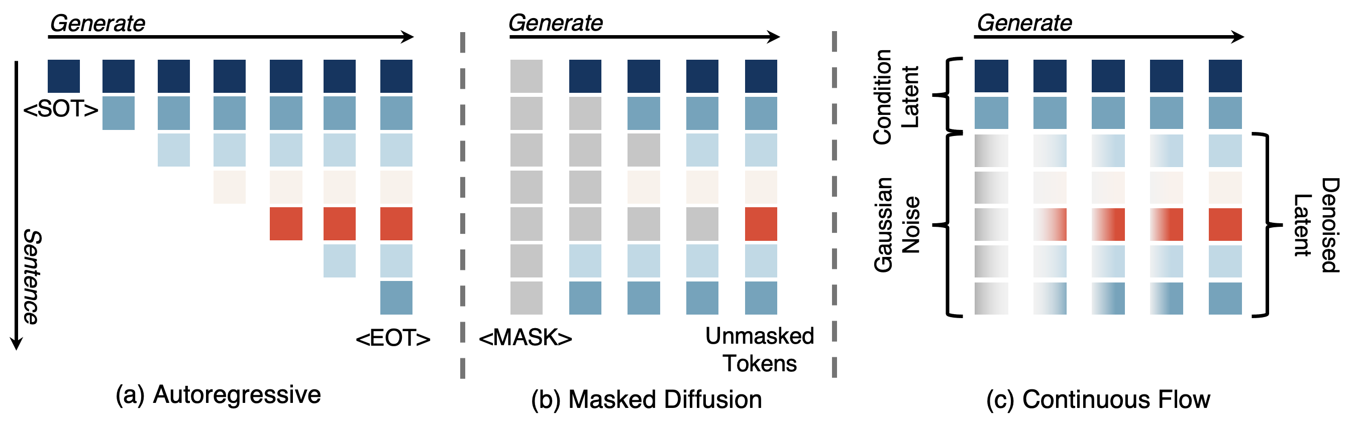
TextLDM has two stages, mirroring Stable Diffusion / DiT for images.
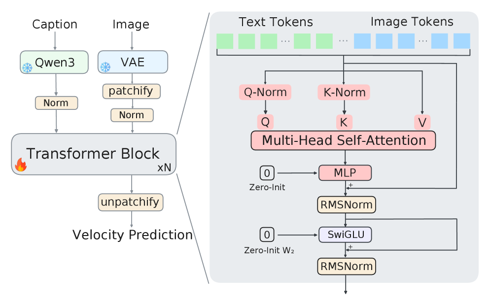
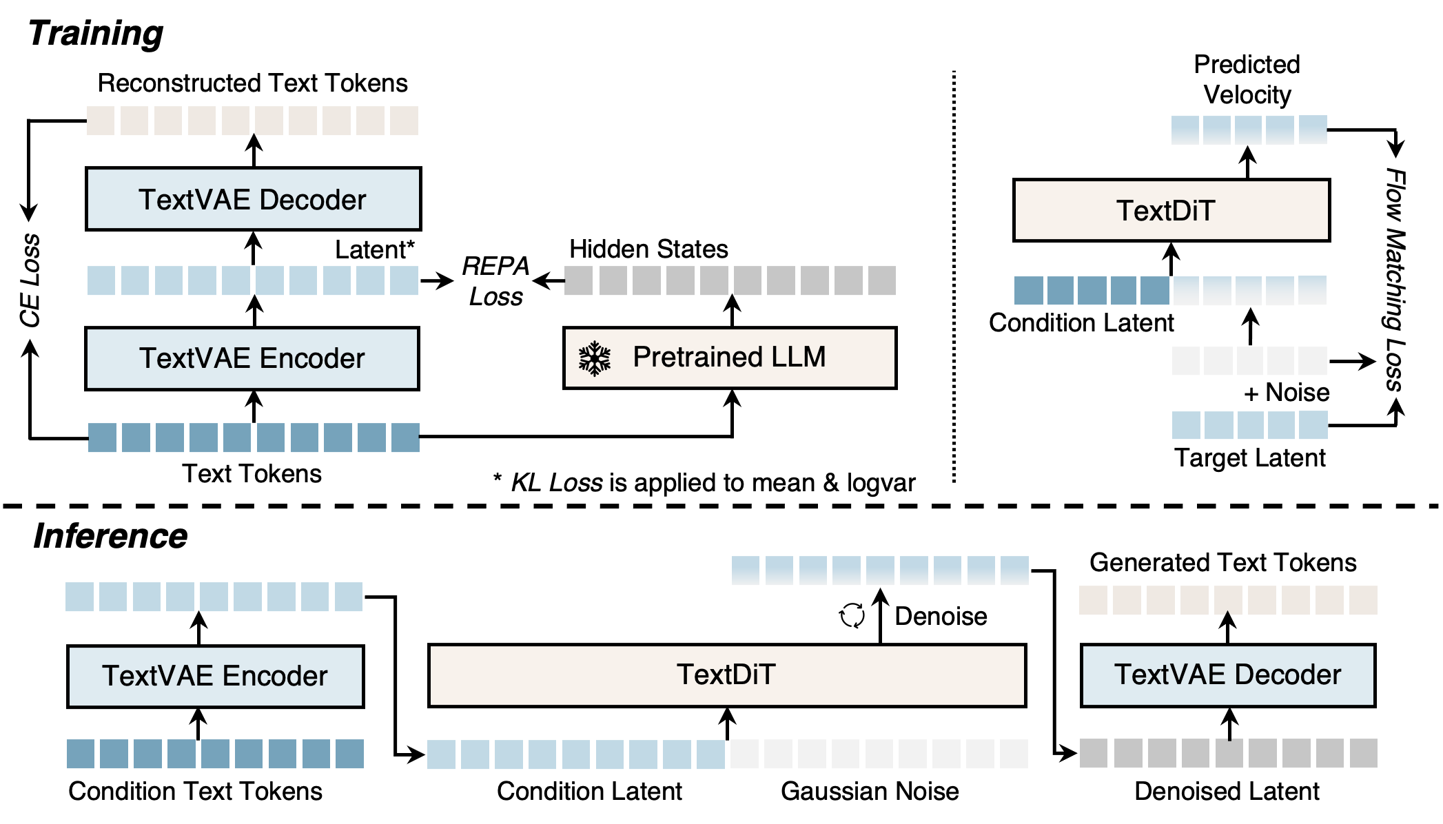
Stage 1 — TextVAE. Tokenize with the Qwen3 tokenizer to \mathbf{x}=(x_1,\dots,x_N). A Transformer encoder E_\phi produces a diagonal Gaussian posterior per position, q_\phi(\mathbf{z}_i\mid \mathbf{x}) = \mathcal{N}(\boldsymbol\mu_i, \boldsymbol\sigma_i^2), with reparameterized samples \mathbf{z}_i = \boldsymbol\mu_i + \boldsymbol\sigma_i\odot\boldsymbol\epsilon. Crucially, the mapping is one-to-one in length — each token gets one latent \mathbf{z}_i\in\mathbb{R}^d — unlike PLAID/TEncDM which compress to a shorter latent sequence. A Transformer decoder D_\psi reconstructs token distributions non-autoregressively under cross-entropy. Training combines reconstruction CE, a KL regularizer on the posterior, and the key ingredient: REPA alignment, which pushes encoder hidden states to match features from a frozen Qwen3-1.7B. Random truncation of input sequences during VAE training teaches the encoder to handle variable lengths, important because the downstream DiT will encode context and target segments independently.
Stage 2 — TextDiT. A standard DiT, identical in architecture to the visual variant, performs flow matching in the latent space. Clean context latents \mathbf{z}^{\text{ctx}} and noisy target latents \mathbf{z}^{\text{tgt}}_t are concatenated; the network predicts the velocity field v_\theta that transports \mathcal{N}(0,I) to the data-conditional distribution, with the standard FM loss \mathcal{L}_{\text{FM}} = \mathbb{E}_{t,\mathbf{z}_0,\mathbf{z}_1}\big\|v_\theta(\mathbf{z}_t,t,\mathbf{z}^{\text{ctx}}) - (\mathbf{z}_1-\mathbf{z}_0)\big\|^2, with \mathbf{z}_t=(1-t)\mathbf{z}_0 + t\mathbf{z}_1. Unconditional generation drops the context. To prevent target-into-context leakage during training, context and target are encoded separately by E_\phi rather than encoding the full sequence and slicing.
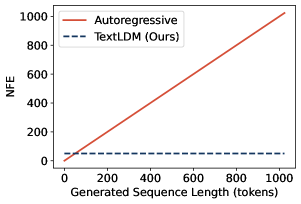
A practical consequence of operating on a fixed-length latent grid is that decoding cost is decoupled from sequence length: the number of function evaluations (NFE) is set by the FM solver, not by N. The authors report length-invariant NFE up to 1024 tokens, in contrast to AR’s linear scaling.
Results
Trained from scratch on OpenWebText2 under matched settings, TextLDM substantially outperforms prior diffusion language models and matches GPT-2. The headline claim — that REPA, not reconstruction fidelity, is the binding constraint on continuous-latent text diffusion — is supported by ablations: a VAE with low reconstruction error but no LM-feature alignment yields poor downstream generation, while alignment to Qwen3-1.7B features rescues quality. This contradicts the implicit assumption in earlier text-VAE work that pushing CE reconstruction lower is sufficient.
Limitations and open questions
- The paper trains on OpenWebText2 against GPT-2-class baselines; whether the recipe scales to modern LLM regimes (10B+ parameters, multi-trillion-token corpora) is unverified, and REPA against Qwen3-1.7B effectively distills from a stronger model, complicating same-compute comparisons.
- One-to-one token-to-latent mapping preserves length but discards the compression that made image latent diffusion attractive; the latent dimensionality d and KL weight trade-offs are not deeply explored.
- The non-autoregressive decoder must reconstruct tokens in parallel from possibly imperfect denoised latents; error modes (off-by-one drift, repetition under FM sampling) and the gap between teacher-forced VAE reconstruction and end-to-end generation deserve more analysis.
- Reliance on a pretrained LM for REPA raises a chicken-and-egg question: can a continuous text latent be learned from scratch, or does it fundamentally require an AR teacher?
Why this matters
If continuous latent diffusion can match AR language modeling at GPT-2 scale, the architectural barrier separating visual generation (DiT + FM in a VAE latent) from text becomes negotiable, opening a path to a single backbone for both modalities with length-invariant inference cost. The non-trivial finding — that the latent space, not the diffusion objective, is what has been holding text diffusion back — reframes where future effort should go.
Source: https://arxiv.org/abs/2605.07748
Rethinking State Tracking in Recurrent Models Through Error Control Dynamics
Problem
The literature on state tracking in recurrent architectures has been dominated by expressivity questions: can a given architecture realize a target symbolic transition rule on G? This paper argues that expressivity is necessary but insufficient. What also matters is error control: the dynamics of hidden-state drift along directions that distinguish symbolic states. A model can be expressive enough to encode every state g\in G with a representation c_g\in\mathbb{F}^d, yet fail to track over long horizons because perturbations along the symbolic subspace \mathcal{U}:=\operatorname{span}\{c_g - c_{g'}:g,g'\in G\} do not contract. This is precisely the regime where SSMs and linear-attention variants live, and it explains why benchmark length-generalization on group word problems is so brittle.
Method and core theorem
The central object is the return map F_s = F_{x_T}\circ\cdots\circ F_{x_1} induced by a state-preserving sequence s (i.e., one whose symbolic action T_s is the identity on G). Exact realization requires F_s(c_g)=c_g for all g. The paper then proves:
Theorem 1 (Affine neutrality). If F_s(h)=A_s h + b_s is affine, the representations \{c_g\} are non-degenerate, and F_s(c_g)=c_g for all g, then A_s|_{\mathcal{U}} = I.
The proof is short: differences c_g - c_{g'} span \mathcal{U} and are fixed by F_s, so A_s acts as identity on a spanning set. The consequence is sharp: F_s(c_g + \delta) - F_s(c_g) = \delta \quad \text{for all } \delta\in\mathcal{U}.
So any affine recurrent model — Mamba, Mamba-3, AUSSM, linear RNNs, token-gated RNNs (whose gate depends only on x_t, leaving the update affine in h_{t-1}) — that exactly realizes the symbolic transition cannot have a contracting attractor along the very directions that matter for discrimination. Realization and correction are mutually exclusive on \mathcal{U} for affine models.
State-dependent maps escape this. Writing the local map around c_g as p\mapsto F_s(c_g+p)-c_g, if its Jacobian at p=0 has spectral norm uniformly below one, perturbations along \mathcal{U} contract. State-dependence is necessary, not sufficient — the choice of nonlinearity has to actually deliver Jacobian contraction.
Predictive consequence: finite-horizon tracking
Because affine models cannot contract along \mathcal{U}, within-class spread r_{\mathrm{err}}(t) accumulates while between-class separation r_{\mathrm{sep}}(t) is fixed by the symbolic action. Tracking remains readable only while the distinguishability ratio q(t) = R(t)/M(t) stays below the decoder’s readability threshold (the nearest-centroid bound is q=1/2). The horizon at which q(t) crosses this threshold predicts the maximum length at which test accuracy holds.
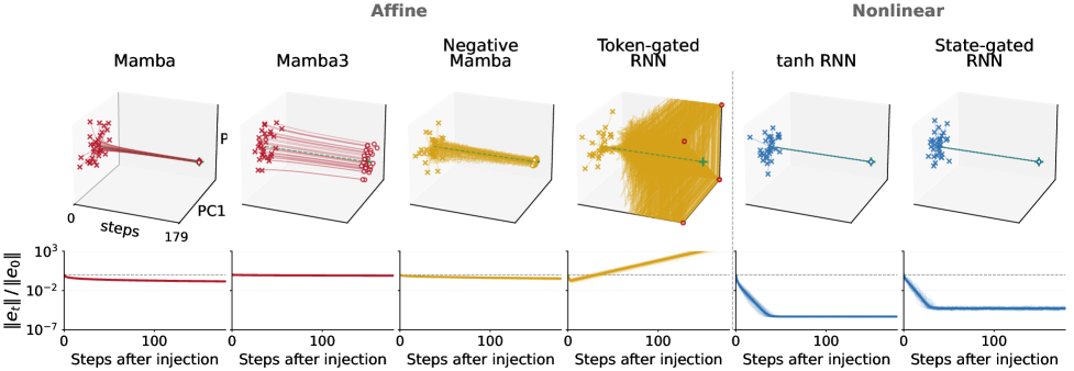
Figure 1 shows the perturbation experiment on S_3: after a noise injection, affine models either globally decay (Mamba, Mamba-3, Negative Mamba — but uniformly, including along non-symbolic directions, which is not the same as correction on \mathcal{U}) or globally expand (Token-gated RNN). Only the state-dependent tanh RNN and State-gated RNN exhibit error contraction concentrated where it matters.
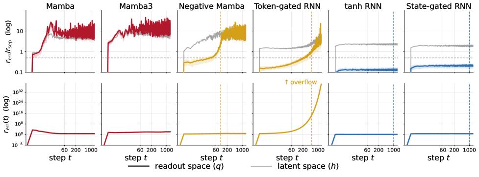
Figure 2 makes the prediction quantitative: each affine model’s empirical max-passing length \mathrm{mp} from Table 2 lines up with where q(t) crosses the 1/2 bound. The state-dependent models keep q(t) bounded indefinitely.
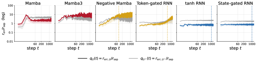
Figure 3 decomposes spread into q_{\mathcal{U}}(t) and q_{\mathcal{U}^\perp}(t), confirming that for affine models the failure is specifically along \mathcal{U}, exactly as Theorem 1 predicts.
Quantitative results
Training is at length \le 60; evaluation extends to length 1000. Cells reporting 60 indicate models that survive only at the curriculum length; ✗ means \mathrm{mp}=0.
- On C_2 (1-layer): vanilla Mamba and Linear RNN fail (✗); Mamba-3 reaches 200; AUSSM and Negative Mamba reach 1000; Token-gated RNN reaches 1000.
- On C_6 (1-layer): all affine models cap at \le 300 (Token-gated RNN), with Mamba and Linear RNN at ✗.
- On S_3 (non-abelian, harder): every affine model fails to extrapolate at L1 except Negative Mamba (100) and Token-gated RNN (500). Two-layer stacks help marginally (Token-gated RNN reaches 1000).
- The state-dependent tanh RNN and State-gated RNN reach 1000 on every task, every depth.
The Token-gated RNN is the cleanest stress test of the theorem: it has rich gating, but because the gate depends only on x_t the update is still affine in h_{t-1}, and it inherits the finite-horizon failure mode despite reaching 500–1000 on easier tasks.
Limitations and open questions
The theorem is about exact affine realization; in practice models are trained to approximate, and “global contraction” affine models like Mamba decay errors along \mathcal{U} at the cost of also decaying \mathcal{U}^\perp and not exactly fixing \{c_g\}. The framework predicts horizons but does not prescribe how much state-dependence is needed, nor which nonlinearities give Jacobian contraction in deep stacks. Group word problems are a controlled probe; whether q(t) predicts failures in less structured tasks (e.g., language modeling regimes that implicitly require state tracking) is open. Finally, the analysis is per-layer; depth allows non-affine compositions even from affine blocks, and the modest L1\toL2 gains hint at this without quantifying it.
Why this matters
Expressivity arguments have been used to defend SSMs and linear attention as adequate for state tracking, but this paper shows that any affine recurrence faces a structural impossibility: it cannot simultaneously fix symbolic representations and contract perturbations between them. The distinguishability ratio gives a model-agnostic, predictive horizon for when tracking will collapse, reframing “length generalization” as an error-control problem rather than an architectural-capacity problem.
Source: https://arxiv.org/abs/2605.07755
MACE-Dance: Motion-Appearance Cascaded Experts for Music-Driven Dance Video Generation
Problem
Music-driven dance video generation requires jointly producing kinematically plausible, musically synchronized human motion and a spatiotemporally coherent rendering that preserves the identity in a reference image. Prior approaches address only fragments of the pipeline: music-to-3D-motion methods (EDGE, Lodge) ignore appearance; pose-driven animators (e.g., Hallo2, Echomimic-V3, WAN-S2V) require an externally supplied driving signal and cannot be conditioned directly on music. Direct music-to-video learning suffers from spurious cross-modal correlations because audio carries weak signal about pixel-level appearance.
Method
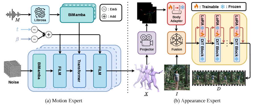
MACE-Dance factorizes p(D \mid M, I) into a cascade of two experts via an explicit 3D motion bottleneck X \in \mathbb{R}^{T \times C_x} in SMPL parameters:
p(D \mid M, I) = \int p_{\text{AE}}(D \mid X, I)\, p_{\text{ME}}(X \mid M)\, dX.
The authors argue 3D over 2D keypoints because (i) global translation/orientation are preserved, (ii) supervision is decoupled from camera and body proportions, and (iii) self-occlusion is handled implicitly. Hands are dropped (SMPL, not SMPL-X) since body-only motion is sufficient at current data scale.
Motion Expert (ME). A diffusion model with a BiMamba–Transformer hybrid backbone: 2 BiMamba layers with a Genre-Gate process the music conditioning, followed by 8 BiMamba-Transformer blocks producing the motion vector. Mamba units use state size 16, kernel 4, expansion 2, latent 512; Transformer blocks use 4 heads, FFN 1024, dropout 0.1, GELU. Training combines reconstruction, 3D joint position, velocity, and foot-contact losses with weights \lambda_{rec}=0.636, \lambda_{joint}=0.636, \lambda_{vel}=2.964, \lambda_{foot}=10.942. Trained on FineDance for 4000 epochs, batch 128, Adam lr 4\times 10^{-4}, weight decay 0.02, EMA decay 0.9999, on 8 H20 GPUs. Training sequences are 240 frames (8 s); inference extends to 1024 frames (34.13 s).
Crucially, ME uses Guidance-Free Training (GFT), replacing classifier-free guidance with a \beta-conditioned model interpolating between conditional and unconditional behavior, so that a single forward pass at inference attains a chosen point on the diversity–fidelity curve. The ablation in Table 7 verifies the trade-off: \beta=1.00 gives the highest diversity (\mathrm{DIV}_k=13.29, \mathrm{DIV}_g=9.68) but worst fidelity (\mathrm{FID}_k=29.35, \mathrm{FID}_g=31.91); \beta=0.50 flips it (\mathrm{FID}_k=15.11, \mathrm{FID}_g=24.15, \mathrm{DIV}_k=8.64, below the GT 9.94); \beta=0.00 is numerically unstable (NaN). The default \beta=0.75 yields \mathrm{FID}_k=17.83, \mathrm{FID}_g=25.09, \mathrm{DIV}_k=10.30, \mathrm{DIV}_g=8.09, \mathrm{BAS}=0.229 — diversity above ground truth and substantially better fidelity than \beta=1.00.
Motion editing. Because ME operates on structured 3D motion, masked DDIM denoising,
\tilde{z}_{t-1} = m \odot q(x^{\text{known}}, t-1) + (1-m) \odot \hat{z}_{t-1},
supports temporal in-betweening, joint-wise inpainting (e.g., fix upper body, regenerate lower), and trajectory-guided generation (constrain root translation), all without retraining.
Appearance Expert (AE). A motion- and reference-conditioned video synthesizer with a “decoupled kinematic” design (the abstract is truncated in the provided text). It consumes the SMPL sequence X and reference I, and is trained on the full MA-Data corpus rather than the motion-centric subset.
Data
The authors curate MA-Data: 70k clips, 5–10 s each, totaling 116 hours across 20+ dance genres. Two complementary subsets: (i) 20k clips (~28 h) of FineDance motion retargeted to a character and rendered front-view (motion-centric, used to train ME), and (ii) 50k in-the-wild internet clips (~88 h) cleaned via TransNet V2 shot detection, optical-flow magnitude filtering for static clips, and ViTPose single-performer enforcement (appearance-centric). A separate test set of 200 5-s TikTok clips is held out.
Results
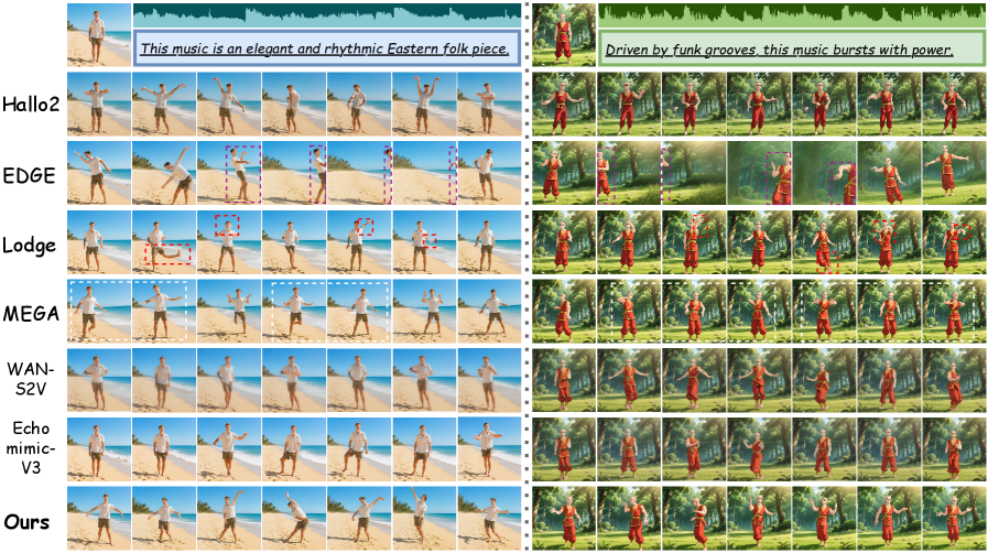
In a preference-based user study with 40 dance-trained participants on 30 8-s music segments, MACE-Dance is preferred over Hallo2, EDGE, Lodge, WAN-S2V, and Echomimic-V3 across all six dimensions — DS, DQ, DC (motion) and PQ, TC, IC (appearance). Qualitatively, baselines exhibit characteristic failure modes: Hallo2 blurs faces and adds background artifacts; EDGE shows abrupt motion discontinuities; Lodge generates physically implausible poses; WAN-S2V and Echomimic-V3 produce repetitive, low-amplitude motion. MACE-Dance maintains coherent appearance and expressive motion across real-person and anime references and across Eastern Folk vs. Popping music.
Limitations and open questions
- ME is body-only (SMPL, no hands/face); fingers and facial micro-motion — important for genres like Latin or K-pop — are not modeled.
- ME and AE are trained on disjoint data subsets, so error propagation across the cascade is not explicitly minimized; AE inherits whatever artifacts ME’s SMPL trajectory contains.
- The user study uses preference selection rather than absolute scoring, so effect sizes vs. each baseline are not quantified per dimension in the provided text.
- No quantitative video-level metrics (FVD, identity similarity, temporal consistency) are reported in the excerpts; appearance evaluation rests primarily on user preference.
- Identity preservation in AE creates obvious deepfake misuse risk; the authors flag this but propose only generic safeguards (watermarking, provenance).
- Long-horizon coherence: ME generates 1024-frame sequences but training is 240-frame, leaving the extrapolation regime untested quantitatively.
Why this matters
The cascade enforces a clean separation between music-conditioned motion semantics and identity-conditioned rendering, with explicit 3D motion as the interface — this both removes the need for paired (music, video, identity) supervision at the appearance stage and yields a reusable motion asset transferable to rigs, avatars, or humanoid control. GFT replacing CFG in motion diffusion is a concrete demonstration that a \beta-indexed family of diversity–fidelity trade-offs can be learned in one model on a non-text generative task.
Source: https://arxiv.org/abs/2512.18181
Hacker News Signals
LLMs corrupt your documents when you delegate
Source: https://arxiv.org/abs/2604.15597
This paper documents a systematic failure mode: when LLMs are used as agents to edit, summarize, or otherwise transform documents on a user’s behalf, they introduce unauthorized semantic changes—rewording, omitting, or subtly altering content beyond the delegated task. The authors call this “document corruption” and frame it as distinct from hallucination: the model is not fabricating facts about the world, it is faithfully completing an agentic task while silently degrading the source material.
The study evaluates several frontier models (GPT-4o, Claude 3.x, Gemini 1.5) on a benchmark of document manipulation tasks—copy-editing, reformatting, translation, summarization with retention instructions—and measures divergence from the original at the lexical, semantic, and factual levels. The core finding is that models systematically over-edit: even when explicitly instructed to preserve content, they paraphrase, condense, and restructure. The divergence is not random; it correlates with model capability—stronger models corrupt more fluently, making the changes harder to detect.
The mechanism proposed is that instruction-tuned models are trained to be “helpful,” which in practice means producing polished output, and this training objective conflicts with strict fidelity constraints. The RLHF reward signal does not penalize smooth paraphrase, so models learn that rewriting is acceptable by default.
The paper proposes a fidelity-aware evaluation metric combining token-level edit distance with semantic similarity (using embedding cosine distance) and factual consistency scores from an NLI model. Under this metric, all tested models score substantially below human editors given equivalent instructions.
Practically this is a serious concern for agentic pipelines doing document processing at scale—legal, medical, or archival contexts where verbatim fidelity matters. The paper does not propose a training fix, leaving open how to instill genuine fidelity constraints without compromising general capability. Prompting mitigations (explicit diff-only instructions, structured output formats) reduce but do not eliminate corruption.
How Fast Does Claude, Acting as a User Space IP Stack, Respond to Pings?
Source: https://dunkels.com/adam/claude-user-space-ip-stack-ping/
Adam Dunkels (author of uIP and lwIP) prompted Claude to implement a user-space IP stack in Python and then benchmarked ICMP echo round-trip latency against that stack. The technical substance is more interesting than the stunt framing suggests.
Claude generated a functional raw-socket-based Python implementation handling Ethernet frame parsing, IP header construction (with checksum calculation), and ICMP echo reply generation—roughly the core of what uIP does in a few hundred lines of C, reproduced in Python from a prompt. Dunkels verified correctness by actually sending pings from another host and receiving replies.
The latency numbers are predictably large: round-trip times in the hundreds of milliseconds to low seconds, dominated entirely by LLM inference time per token rather than anything network-related. A real user-space stack like DPDK or even lwIP running on an embedded MCU at 8 MHz answers pings in under a millisecond. The comparison is obviously not serious benchmarking.
What is technically notable is the code quality: the generated stack correctly handles IP checksum computation (one’s complement sum over the header words), parses variable-length IP options, and constructs valid ICMP type-0 replies by swapping src/dst and recomputing the ICMP checksum. These are the kinds of bit-level details that naive code generation often gets wrong. Dunkels notes one subtle bug—the TTL field was not decremented, which is correct behavior for an end host but would be wrong for a router—suggesting the model understood the semantic context.
The broader technical point is about LLMs as protocol implementation tools: for low-stakes or prototyping contexts, a model can produce structurally correct network code from a high-level description. The failure modes are subtle (off-by-one in header offsets, endianness) rather than structural, which matches what you would expect from a model trained on abundant RFC and networking code.
Killswitch: Per-function short-circuit mitigation primitive
Source: https://lwn.net/ml/all/20260507070547.2268452-1-sashal@kernel.org/
This Linux kernel patch series from Sasha Levin proposes a killswitch mechanism: a per-function binary flag that, when set, causes that function to return immediately (short-circuit) without executing its body. The intent is a lightweight, runtime-controllable mitigation primitive for known-vulnerable functions that cannot be safely removed from the kernel image but need to be disabled in response to active exploits or during debugging.
The implementation works by patching a function’s prologue at runtime with a conditional branch to an early return, similar in spirit to static calls and jump labels but with the added semantic that the function returns a safe default value (zero/NULL) rather than an error code. This is distinct from existing mechanisms like ftrace (which has higher overhead) or static_key (which requires recompilation to add). The killswitch can be toggled via a sysfs interface or from the kernel command line.
The mechanical implementation uses text patching: at boot, a NOP is emitted at the function entry; when the killswitch is activated, that NOP is replaced with a jump to a trampoline that executes a ret with a zeroed return value. On x86 this is a 5-byte near jump. The patch relies on text_poke_bp, the existing BP-based patching mechanism used by jump labels, ensuring correctness on SMP systems.
Open questions include the semantic contract for callers: a function returning 0/NULL instead of an error code may cause callers to proceed as if success occurred, potentially creating new failure modes. The RFC discussion on the list raises exactly this: in some cases a panic or explicit error return would be safer than a silent zero. There is also the question of interaction with lockdep and RCU—functions that acquire locks or perform RCU reads cannot simply be short-circuited without leaving kernel state inconsistent.
Hardening Firefox with Claude Mythos Preview
Source: https://hacks.mozilla.org/2026/05/behind-the-scenes-hardening-firefox/
Mozilla describes using Anthropic’s Claude Mythos Preview (a coding-focused model variant) to assist with security hardening of Firefox’s C++ codebase at scale. The technical work involves two categories: automated identification and remediation of unsafe memory patterns, and generation of fuzzing harnesses.
For memory safety, the workflow feeds Claude sections of C++ source alongside a set of hardening rules (preferring mozilla::Span over raw pointer+length pairs, replacing manual new/delete with UniquePtr, flagging unchecked integer arithmetic in size calculations). Claude proposes diffs; engineers review and land them. Mozilla reports processing tens of thousands of lines across core components including the layout engine and IPC layer. The value-add over static analyzers like clang-tidy is that Claude can handle refactors that require understanding calling context—e.g., propagating a Span through three layers of call stack rather than just flagging the leaf function.
For fuzzing, Claude generates LLVMFuzzerTestOneInput harnesses given a function signature and doc comment. This is largely a template-filling task but the interesting part is that Claude infers input constraints (e.g., a buffer must be null-terminated, a length parameter must be nonzero) from code context rather than explicit specification, producing harnesses that reach deeper code paths than naive random-byte fuzzing.
The post is candid about failure modes: Claude occasionally produces diffs that are syntactically correct but semantically wrong (incorrect lifetime assumptions, missing null checks after the refactor). The human review layer is described as non-negotiable. There is no claim of fully autonomous hardening.
What is not discussed: the rate of false positives from the LLM-proposed diffs, whether the fuzzing harnesses found new bugs, and how Mythos Preview differs architecturally from standard Claude 3.x. The omission of quantitative security outcomes is a notable gap.
Gemini API File Search is now multimodal
Google has extended the Gemini API’s File Search (RAG-over-uploaded-files) capability to support multimodal queries: the retrieval stage can now match against image content, tables, charts, and mixed-modality documents, not just text chunks.
The technical mechanism relies on Gemini’s native multimodal embeddings, which map images, text, and structured data into a shared vector space. At indexing time, uploaded files are chunked and each chunk is embedded with the multimodal encoder; at query time, a text or image query is embedded in the same space and approximate nearest-neighbor search retrieves relevant chunks. Retrieved chunks (including image tiles) are then passed directly to the Gemini context window for answer generation.
The important constraint is that retrieval is still embedding-based similarity search rather than structured search—so queries like “find the bar chart showing Q3 revenue” depend on how well the multimodal embedding captures that semantic content. For charts and diagrams with limited text labels, embedding quality degrades relative to text-dense documents. The system does not extract structured data from charts before embedding; it operates on rendered image patches.
From an API perspective, the interface is unchanged for developers already using File Search: uploaded files are automatically indexed with the new multimodal encoder, and queries return interleaved text and image chunks. The context window budget for retrieved content remains a binding constraint for long documents with many images.
Practical limitations: no support yet for video keyframe retrieval, the ANN index does not expose configuration (HNSW parameters, quantization), and there is no hybrid sparse-dense retrieval option, which typically improves precision for keyword-specific queries. For production RAG systems over heterogeneous document corpora, the lack of BM25-style term matching alongside the dense retrieval is the most significant gap relative to specialized pipelines like Vespa or Weaviate with hybrid search enabled.
Noteworthy New Repositories
raiyanyahya/how-to-train-your-gpt
A ground-up GPT implementation where every line of code carries an inline comment explaining its purpose. The repository walks through the full training stack: tokenization (BPE), embedding layers, multi-head self-attention with causal masking, positional encodings, feed-forward sublayers, layer normalization placement, and a basic training loop with cross-entropy loss. The pedagogical intent is explicit — derivations are not assumed, so the comments explain why the residual stream exists, what the scaling factor \frac{1}{\sqrt{d_k}} in attention achieves, and how weight tying between embedding and unembedding matrices works. The architecture targets a modern GPT-2-class model rather than the original GPT-1 structure, incorporating pre-LayerNorm and learned positional embeddings. For readers building intuition about implementation details that papers gloss over — gradient checkpointing, key-value cache construction during inference, or the exact tensor shapes flowing through a batched attention kernel — this is a useful reference. It does not cover distributed training, FSDP, or flash attention variants, so it is best read alongside more production-oriented codebases rather than as a standalone training recipe.
Source: https://github.com/raiyanyahya/how-to-train-your-gpt
amitshekhariitbhu/llm-internals
A structured curriculum covering LLM internals across several layers of abstraction. The repository progresses from tokenization algorithms (BPE, WordPiece, SentencePiece) through the transformer block in detail — QKV projections, multi-head attention, grouped-query attention (GQA), rotary positional embeddings (RoPE), RMSNorm vs. LayerNorm trade-offs — and into inference-time mechanics such as KV caching, speculative decoding, and quantization strategies (INT8, GPTQ, AWQ). Each topic is documented with equations and annotated code snippets rather than prose alone. The inference optimization section is particularly concrete: it distinguishes prefill and decode phases, explains why memory bandwidth is the binding constraint during autoregressive generation, and shows how continuous batching addresses GPU utilization. The repository does not train models from scratch; it is a reading and reference guide backed by minimal runnable examples. Coverage of post-training (RLHF, DPO) is present but lighter than the architecture sections. Useful for someone who can read a transformer paper but wants the engineering context that papers omit.
Source: https://github.com/amitshekhariitbhu/llm-internals
future-agi/future-agi
An Apache 2.0, self-hostable observability and evaluation platform targeting LLM applications and multi-agent pipelines. The core components are: a tracing layer that instruments LLM calls and agent tool invocations via OpenTelemetry-compatible spans; an evaluation engine that runs both model-based and deterministic scorers against traced outputs; a simulation harness for replaying agent trajectories under controlled conditions; a dataset store for curating and versioning eval sets; an LLM gateway that centralizes routing, credential management, and rate limiting; and a guardrails module for enforcing output constraints at inference time. The architecture separates the data plane (tracing, gateway) from the evaluation plane, so instrumentation overhead does not block the eval pipeline. Self-hosting is supported via Docker Compose with Postgres and a Python backend. The platform is broadly comparable to LangSmith or Weights and Biases Weave in scope, but with a fully open codebase. The simulation component — which supports counterfactual agent runs — is the most differentiated feature relative to existing open-source observability tools.
Source: https://github.com/future-agi/future-agi
oritera/Cairn
Cairn frames autonomous penetration testing as a general-purpose state-space search problem. The agent maintains an explicit state graph where nodes represent system configurations (open ports, discovered credentials, privilege levels) and edges represent actions (exploit attempts, lateral movement steps). Search over this graph is guided by a heuristic function that estimates proximity to the target objective, with support for both depth-first and best-first traversal policies. The LLM component acts as a planner that proposes candidate actions given the current state description; a symbolic verifier checks preconditions before execution. This hybrid design avoids the pure prompt-chaining brittleness of LLM-only agents while retaining flexibility for novel attack surfaces that rule-based systems cannot enumerate. Validation is on standard CTF-style environments and simulated networks rather than live targets. The state-space framing is the substantive contribution: it provides a principled way to handle long-horizon, partially observable tasks where intermediate states must be tracked explicitly. The general-purpose claim — that the same engine applies to domains beyond pentesting — is asserted but not yet demonstrated empirically in the repository.
Source: https://github.com/oritera/Cairn
kyegomez/OpenMythos
A speculative reverse-engineering of Anthropic’s internal “Mythos” framework — the identity, character, and value-alignment scaffolding described in Claude’s publicly released model specification — implemented from first principles. The repository attempts to operationalize concepts from that document (character consistency, corrigibility gradients, the principal hierarchy, Constitutional AI-style self-critique) as concrete training and inference code. Key components include a multi-objective reward model that scores outputs jointly on helpfulness, harmlessness, and honesty with configurable weighting; a debate-style self-critique loop where the model challenges its own draft responses against stated principles; and a principal hierarchy abstraction that distinguishes operator-level and user-level instructions with differential trust. The implementation uses standard transformer fine-tuning and RLHF infrastructure. The star count (12k+) reflects community interest in interpretable alignment scaffolding rather than empirical validation — the repository is explicitly theoretical and no benchmark results against Claude or comparable models are provided. The primary value is as a structured reading of the Claude model spec translated into executable pseudocode, not as a production alignment system.